We know that the average of $f$ over $[x-T,x+T]$ for any fixed $x$ is given by $$f_{\text{avg}}(x)=\frac{1}{2T}\int_{x-T}^{x+T} f(t)\,\mathrm{d}t.$$ Define $\phi=\frac{\Pi_T}{2T}$, where \begin{align}\Pi_T(t)=\begin{cases}1,&\quad -T\leq t\leq T\\
0,&\quad |t|>T.\end{cases}\end{align} We then have $$\int_{-\infty}^\infty \phi(t)\,\mathrm{d}t=\frac{1}{2T}\int_{-T}^T \Pi_T(t)\,\mathrm{d}t=1.$$ For any fixed $x$, \begin{align}\phi(x-t)=\begin{cases}\frac{1}{2T},&\quad x-T\leq t\leq x+T\\
0,&\quad \text{else}.\end{cases}\end{align} Thus, for any given function $f$ and any fixed value of $x$, \begin{align}f(t)\phi(x-t)=\begin{cases}\frac{1}{2T}f(t),&\quad x-T\leq t\leq x+T\\
0,&\quad \text{else}.\end{cases}\end{align} We conclude that $$f_{\text{avg}}(x)=\int_{-\infty}^\infty f(t)\phi(x-t)\,\mathrm{d}t.$$ More generally, when we replace $\phi$ with an arbitrary function, we have the definition of a convolution: the convolution of two functions $f$ and $g$ is given by $$f*g(x)=\int_{-\infty}^\infty f(t)g(x-t)\,\mathrm{d}t.$$ Reference: The Mathematics of Imaging by Timothy G. Freeman
Tuesday, 6 September 2016

Friday, 1 July 2016
Nth root
We first study the sequence $$x_{n+1}=\dfrac{1}{2}(x_n+\dfrac{a}{x_n}),$$ where $a=2,x_1=1$ and examine the numbers $x_2,x_3,x_4,x_5$ : $$x_2=\dfrac{1}{2}(1+2)=1.5\\x_3=\dfrac{1}{2}(1.5+\dfrac{2}{1.5})\approx 1.4167\\x_4=\dfrac{1}{2}(1.4167+\dfrac{2}{1.4167})\approx1.4142\\x_5=\dfrac{1}{2}(1.4142+\dfrac{2}{1.4142})\approx 1.4142\\ \cdots$$ We can show that the sequence tends to $\sqrt{2}$. More generally, take $l=\lim x_n$, so $l=\lim x_{n+1}$ and so\begin{align*}l&=\dfrac{1}{2}(l+\dfrac{a}{l})\\ 2l^2&=l^2+a\\ l&=\sqrt{a}\;\;\text{(reject the negative number because }\;x_n>0).\end{align*} This sequence helps us generate the square root of any positive number. You may ask: how can we come up with such a sequence? The reasoning is as follows: if $x_1\neq \sqrt{a}$, then we have $x_1<\sqrt{a}$ or $x_1>\sqrt{a}$. In the first case, we have $\sqrt{a} x_1<a$ or $\sqrt{a}<\dfrac{a}{x_1}$. In the other case, if $x_1>\sqrt{a}$, then $\sqrt{a}>\dfrac{a}{x_1}$. Therefore, we have $x_1<\sqrt{a}<\dfrac{a}{x_1}$ or $\dfrac{a}{x_1}<\sqrt{a}<x_1$. If we take the average of $x_1$ and $\dfrac{a}{x_1}$, namely $x_2=\dfrac{1}{2}(x_1+\dfrac{a}{x_1})$, then the result will be between $x_1$ and $\dfrac{a}{x_1}$. Repeat this process several times: $$x_3=\dfrac{1}{2}(x_2+\dfrac{a}{x_2}), x_4=\dfrac{1}{2}(x_3+\dfrac{a}{x_3}) \cdots$$ The sequence $(x_n)$ tends to $\sqrt{a}$.
In fact, the sequence for square root can be generalised to one for nth root. $x_{n+1}=\dfrac{1}{p}\bigg((p-1)x_n+\dfrac{a}{x_n^{p-1}}\bigg)$ The reasoning is similar. We consider $\underbrace{x_n\times x_n\times \cdots\times x_n}_{p-1\; times}\times \dfrac{a}{x_n^{p-1}}=a$ and take the average of these $p$ factors.
These sequences are related to the method of Newton-Raphson. Finding the square root is equivalent to solving the equation $x^2-a=0$. Let $f(x)=x^2-a$. Then, $$x_{n+1}=x_n-\dfrac{f(x_n)}{f'(x_n)}=x_n-\dfrac{x_n^2-a}{2x_n}=\dfrac{1}{2}(x_n+\dfrac{a}{x_n}).$$ As for the nth root, we can solve the equation $x^p-a=0$ and we have $$x_{n+1}=x_n-\dfrac{x_n^p-a}{px_n^{p-1}}=x_n-\dfrac{1}{p}x_n+\dfrac{a}{px_n^{p-1}}=\dfrac{1}{p}\bigg((p-1)x_n+\dfrac{a}{x_n^{p-1}}\bigg).$$
In fact, the sequence for square root can be generalised to one for nth root. $x_{n+1}=\dfrac{1}{p}\bigg((p-1)x_n+\dfrac{a}{x_n^{p-1}}\bigg)$ The reasoning is similar. We consider $\underbrace{x_n\times x_n\times \cdots\times x_n}_{p-1\; times}\times \dfrac{a}{x_n^{p-1}}=a$ and take the average of these $p$ factors.
These sequences are related to the method of Newton-Raphson. Finding the square root is equivalent to solving the equation $x^2-a=0$. Let $f(x)=x^2-a$. Then, $$x_{n+1}=x_n-\dfrac{f(x_n)}{f'(x_n)}=x_n-\dfrac{x_n^2-a}{2x_n}=\dfrac{1}{2}(x_n+\dfrac{a}{x_n}).$$ As for the nth root, we can solve the equation $x^p-a=0$ and we have $$x_{n+1}=x_n-\dfrac{x_n^p-a}{px_n^{p-1}}=x_n-\dfrac{1}{p}x_n+\dfrac{a}{px_n^{p-1}}=\dfrac{1}{p}\bigg((p-1)x_n+\dfrac{a}{x_n^{p-1}}\bigg).$$
Saturday, 21 May 2016
Deriving Power Sums by Polynomial Interpolation
Most of us have seen these formulas: $$\sum_{i=k}^n k=1+2+\cdots+n=\dfrac{1}{2}n(n+1)\\ \sum_{i=k}^n k^2=1+4+\cdots+n^2=\dfrac{1}{6}n(n+1)(2n+1)\\ \sum_{i=k}^n k^3=1+8+\cdots+n^3=\dfrac{1}{4}n^2(n+1)^2\\ \sum_{i=k}^n k^4=1+16+\cdots+n^4=\dfrac{1}{30}n(n+1)(2n+1)(3n^2+3n-1).$$ These can be proved by mathematical induction, but we can actually derive them on our own!
We simply acknowledge the following fact: for any positive integer $p$, the power sum $\sum_{k=1}^n k^p$ can always be expressed as a polynomial $f(n)$ that has degree $p+1$ and has rational coefficients.
Let's try to derive the first and the last formula. For the first, let $f(n)=an^2+bn+c$. We have $f(1)=1,f(2)=3,f(3)=6$. We want to solve the linear system: $$a+b+c=1\\ 4a+2b+c=3\\ 9a+3b+c=6,$$ or equivalently in matrix form $$\begin{pmatrix}1&1&1\\ 4&2&1\\ 9&3&1\end{pmatrix}\begin{pmatrix}a\\b\\c\end{pmatrix}=\begin{pmatrix}1\\3\\6\end{pmatrix}.$$ Note that $$\begin{pmatrix}1&1&1\\ 4&2&1\\ 9&3&1\end{pmatrix}$$ is a Vandermonde matrix. Just type invander([1 2 3])\[1;3;6] in Matlab and we have the solution: $a=1/2,b=1/2,c=0$.
For the last formula, let $f(n)=an^5+bn^4+cn^3+dn^2+en+f$. Then $f(1)=1,f(2)=17,f(3)=98,f(4)=354,f(5)=979,f(6)=2275$. Typevander([1 2 3 4 5 6]\[1;17;98;354;979;2275] in Matlab and we have $a=1/5, b=1/2, c=1/3, d=0, e=-1/30, f=0$. Finally, factor(1/5*x^5+1/2*x^4+1/3*x^3-1/30*x) gives the formula. The reader can also try to derive the formulas for $\sum_{i=k}^n k^5$ and $\sum_{i=k}^n k^6$.
We simply acknowledge the following fact: for any positive integer $p$, the power sum $\sum_{k=1}^n k^p$ can always be expressed as a polynomial $f(n)$ that has degree $p+1$ and has rational coefficients.
Let's try to derive the first and the last formula. For the first, let $f(n)=an^2+bn+c$. We have $f(1)=1,f(2)=3,f(3)=6$. We want to solve the linear system: $$a+b+c=1\\ 4a+2b+c=3\\ 9a+3b+c=6,$$ or equivalently in matrix form $$\begin{pmatrix}1&1&1\\ 4&2&1\\ 9&3&1\end{pmatrix}\begin{pmatrix}a\\b\\c\end{pmatrix}=\begin{pmatrix}1\\3\\6\end{pmatrix}.$$ Note that $$\begin{pmatrix}1&1&1\\ 4&2&1\\ 9&3&1\end{pmatrix}$$ is a Vandermonde matrix. Just type in
For the last formula, let $f(n)=an^5+bn^4+cn^3+dn^2+en+f$. Then $f(1)=1,f(2)=17,f(3)=98,f(4)=354,f(5)=979,f(6)=2275$. Type
Sunday, 15 May 2016
Manipulations of Sums
Let $a_1,a_2,\cdots$ be any sequence of numbers. We are often interested in sums such as $a_1+\cdots+a_n$. This sum can be written more compactly using either of the following equivalent notations: $$\sum_{i=1}^n a_i\quad \text{or}\quad \sum_{1\leq i\leq n} a_i.$$ In general, if $R(i)$ is any relation involving $i$, the symbol $$\sum_{R(i)} a_i$$ means the sum of all $a_i$, where $i$ is an integer satisfying the condition $R(i)$. The letter $i$ is a dummy variable or index variable that may be renamed without changing the result.
We now discuss four important algebraic operations on sums.
1) The distributive law, for products of sums $$\bigg(\sum_{R(i)} a_i\bigg)\bigg(\sum_{S(j)} b_j\bigg)=\sum_{R(i)}\bigg(\sum_{S(j)} a_ib_j\bigg)$$ Consider for example $$\begin{align}\bigg(\sum_{i=1}^2 a_i\bigg)\bigg(\sum_{j=1}^3 b_j\bigg)&=(a_1+a_2)(b_1+b_2+b_3)\\
&=(a_1b_1+a_1b_2+a_1b_3)+(a_2b_1+a_2b_2+a_2b_3)\\
&=\sum_{i=1}^2\bigg(\sum_{j=1}^3 a_ib_j\bigg).\end{align}$$ 2) Interchanging order of summation $$\sum_{R(i)}\sum_{S(j)} a_{ij}=\sum_{S(j)}\sum_{R(i)} a_{ij}$$ For example, $$\sum_{R(i)}\sum_{j=2}^2 a_{ij}=\sum_{R(i)}(a_{i1}+a_{i2})\\ \sum_{j=1}^2 \sum_{R(i)} a_{ij}=\sum_{R(i)} a_{i1}+\sum_{R(i)} a_{i2}.$$ This means that $$\sum_{R(i)}(b_i+c_i)=\sum_{R(i)}b_i+\sum_{R(i)}c_i,$$ where $b_i=a_{i1}$ and $c_i=a_{i2}$. This operation is very useful because we often know a simple form for $\sum_{R(i)} a_{ij}$ but not for $\sum_{S(j)} a_{ij}$. More generally, we have $$\sum_{R(i)}\sum_{S(i,j)}a_{ij}=\sum_{S'(j)}\sum_{R'(i,j)}a_{ij},$$ where $S'(j)$ is the relation 'there is an integer $i$ s.t. both $R(i)$ and $S(i,j)$ are true'; and $R'(i,j)$ is the relation 'both $R(i)$ and $S(i,j)$ are true'. For example, if the summation is $\sum_{i=1}^n\sum_{j=1}^i a_{ij}$, then $S'(j)$ is the relation 'there is an integer $i$ s.t. $1\leq i\leq n$ and $1\leq j\leq i$, namely $1\leq j\leq n$; and $R'(i,j)$ is the relation '$1\leq i\leq n$ and $1\leq j\leq i$', namely $j\leq i\leq n$. Thus, $$\sum_{i=1}^n\sum_{j=1}^i a_{ij}=\sum_{j=1}^n\sum_{i=j}^n a_{ij}.$$ 3) Change of variable
$$\sum_{R(i)} a_i=\sum_{R(j)} a_j=\sum_{R(p(j))} a_{p(j)}$$ The first equality holds because we are simply changing the dummy variable. In the second case, $p(j)$ is a function of $j$ that represents a permutation of the range. For each integer $i$ satisfying the relation $R(i)$, there is a unique integer $j$ satisfying the relation $p(j)=i$. This condition is always satisfied in cases $p(j)=c+j$ and $p(j)=c-j$, where $c$ is an integer not depending on $j$. For instance, $$\sum_{1\leq i\leq n} a_i=\sum_{1\leq i-1\leq n} a_{i-1}=\sum_{2\leq i\leq n+1} a_{i-1}.$$ Note that for infinite sums, replacing $j$ by $p(j)$ is valid iff $\sum_{R(j)}|a_j|$ exists.
4) Manipulating the domain
If $R(i)$ and $S(i)$ are arbitrary relations, we have $$\sum_{R(i)}a_i+\sum_{S(i)}a_i=\sum_{R(i)\;\text{or}\;S(i)}a_i+\sum_{R(i)\;\text{and}\;S(i)}a_i.$$ For example, $$\sum_{1\leq i\leq m}a_i+\sum_{m\leq i\leq n}a_i=\bigg(\sum_{1\leq i\leq n}a_i\bigg)+a_m,$$ assuming that $1\leq m\leq n$.
Examples from high school:
[The sum of a geometric progression] Assume that $r\neq 1,n\geq 0$. A conventional way of deriving the formula is to consider $S=a+ar+\cdots+ar^n$ and $S-rS$. $$a+ar+\cdots+ar^n\\ \underline{-)\; ar+ar^2+\cdots+ar^{n+1}}\\ a-ar^{n+1}=S(1-r)\\ \Rightarrow S=a\dfrac{1-r^{n+1}}{1-r}$$ This can be easily derived too by manipulating sums: $$\begin{align}a+ar+\cdots+ar^n&=a+\sum_{i=1}^n ar^i\\
&=a+r\sum_{i=1}^n ar^{i-1}\\
&=a+r\sum_{i=0}^{n-1} ar^i\\
&=a+r\sum_{i=0}^n ar^i-ar^{n+1}\\
&=a\dfrac{1-r^{n+1}}{1-r}\end{align}$$
[The sum of a arithmetic progression] Assume $n\geq 0$. Then $$\begin{align}a+(a+d)+\cdots+(a+nd)&=\sum_{i=0}^n (a+di)\\
&=\sum_{n-i=0}^n (a+d(n-i))\\
&=\sum_{i=0}^n (a+dn-di)\\
&=\sum_{i=0}^n (2a+dn)-\sum_{i=0}^n (a+di)\\
&=(n+1)(2a+dn)-\sum_{i=0}^n (a+di)\\
&=a(n+1)+\dfrac{1}{2}dn(n+1)\\
&=\dfrac{1}{2}(n+1)(2a+dn)\end{align}$$ Another example:
Let $$\begin{align}S&=\sum_{i=0}^n\sum_{j=0}^i a_ia_j\\
&=\sum_{j=0}^n\sum_{i=j}^n a_ia_j\\
&=\sum_{i=0}^n\sum_{j=i}^n a_ia_j
\end{align}$$ Then $$\begin{align}2S&=\sum_{i=0}^n\bigg(\sum_{j=0}^i a_ia_j+\sum_{j=i}^n a_ia_j\bigg)\\
&=\sum_{i=0}^n\bigg((\sum_{j=0}^n a_ia_j)+a_ia_i\bigg)\\
&=\bigg(\sum_{i=0}^n a_i\bigg)^2+\bigg(\sum_{i=0}^n a_i^2\bigg)\end{align}$$ We have derived the identity $$\sum_{i=0}^n\sum_{j=0}^i a_ia_j=\dfrac{1}{2}\bigg(\bigg(\sum_{i=0}^n a_i\bigg)^2+\bigg(\sum_{i=0}^n a_i^2\bigg)\bigg).$$
Examples in analysis
In Riemann integration, we have the following result: Suppose $f\in \mathscr{R}[a,b]$ and $g\in \mathscr{C}([m,M])$, where $M=\sup\{f(x)\mid a\leq x\leq b\}$ and $m=\inf\{f(x)\mid a\leq x\leq b\}$. Then $g\circ f\in \mathscr{R}[a,b]$.
Idea: Consider continuous points and discontinuous points separately.
Proof: Let $\varepsilon>0$. Since $g$ is uniformly continuous on $[m,M]$, there exists $\delta>0$ s.t. $|g(x)-g(y)|<\varepsilon$ as $x,y\in [m,M]$ and $|x-y|<\delta$. Also, since $f\in \mathscr{R}[a,b]$, there exists a partition $P=\{x_0,x_1,\cdots,x_n\}$ of $[a,b]$ s.t. $U(f,P)-L(f,P)<\varepsilon \delta$. Consider $A=\{i\mid osc(f)< \delta\}$ (index w.r.t. continuous points) and $A^c=\{i\mid osc(f)\geq \delta\}$ (index w.r.t. discontinuous points). $i\in A$ does not cause much trouble. To handle $i\in A^c$, consider $$\begin{align}\sum_{i\in A^c}(x_i-x_{i-1})&=\dfrac{1}{\delta}\sum_{i\in A^c}\delta (x_i-x_{i-1})\\
&\leq \dfrac{1}{\delta}\sum_{i=1}^n(M_i(f)-m_i(f))(x_i-x_{i-1})\\
&=\dfrac{1}{\delta}(U(f,P)-L(f,P))\\
&<\varepsilon. \end{align}$$Therefore, $$\begin{align}U(g\circ f,P)-L(g\circ f,P)&=\sum_{i=1}^n\bigg(\sup_{[x_{i-1},x_i]}(g\circ f)-\inf_{[x_{i-1},x_i]}(g\circ f)\bigg)(x_i-x_{i-1})\\
&=\sum_{i\in A}\bigg(\sup_{[x_{i-1},x_i]}(g\circ f)-\inf_{[x_{i-1},x_i]}(g\circ f)\bigg)(x_i-x_{i-1})\\&+\sum_{i\in A^c}\bigg(\sup_{[x_{i-1},x_i]}(g\circ f)-\inf_{[x_{i-1},x_i]}(g\circ f)\bigg)(x_i-x_{i-1})\\
&\leq \varepsilon \sum_{i\in A}(x_i-x_{i-1})+C\sum_{i\in A^c}(x_i-x_{i-1})\\
&\leq \varepsilon(b-a)+C\varepsilon\\
&=(b-a+C)\varepsilon,\end{align}$$ where $C=\max\{g(u)\mid m\leq u\leq M\}-\min\{g(u)\mid m\leq u\leq M\}$. It follows that $g\circ f\in \mathscr{R}[a,b]$. $\Box$
Say we want to evaluate $\sum_{n=1}^\infty \dfrac{2n-1}{2^n}$ (which is convergent by ratio test). Consider $$\begin{align}s_n&=\sum_{k=1}^n \dfrac{2k-1}{2^k}\\
&=\dfrac{1}{2}+\sum_{k=2}^n\bigg(\dfrac{2k-1}{2^k}-\dfrac{2k-3}{2^k}\bigg)+\sum_{k=2}^n \dfrac{2k-3}{2^k}\\
&=\dfrac{1}{2}+\sum_{k=2}^n\dfrac{1}{2^{k-1}}+\sum_{k=2}^n \dfrac{2k-3}{2^k}\\
&=\dfrac{1}{2}+\sum_{k=2}^n\dfrac{1}{2^{k-1}}+\sum_{k=2}^n \dfrac{2(k-1)-1}{2^{k-1+1}}\\
&=\dfrac{1}{2}+\sum_{k=2}^n\dfrac{1}{2^{k-1}}+\sum_{k=1}^{n-1} \dfrac{2k-1}{2^{k+1}}\\
&=\dfrac{1}{2}+\sum_{k=2}^n\dfrac{1}{2^{k-1}}+\dfrac{1}{2}s_n-\dfrac{2n-1}{2^n}\\
&=1+2\bigg(1-\dfrac{1}{2^{n-1}}\bigg)-\dfrac{2n-1}{2^n}\end{align}$$ As $n\to \infty$, $s_n\to 3$.
Many manipulations of sums and other formulas become significantly simpler if we use the bracket notation: $$[\text{statement}]=\begin{cases} 1,\quad \text{if the statement is true;}\\ 0,\quad \text{if the statement is false.}\end{cases}$$ Then we can write $$\sum_{R(i)} a_i=\sum_i a_i[R(i)]$$ since the terms of that infinite sums are zero when $R(i)$ is false. In fact, we have seen this expression before -- Kronecker delta symbol is a special case of bracket notation: $$\delta_{ij}=[i=j]=\begin{cases}1,\quad \text{if }i=j\\ 0,\quad \text{if }i\neq j\end{cases}.$$ With bracket notation, we can derive rule (3) from rule (1) and (2): $$\begin{align}\sum_{R(p(j))} a_{p(j)}&=\sum_j a_{p(j)}[R(p(j))]\\
&=\sum_j \sum_i a_i [R(i)][i=p(j)]\\
&=\sum_i a_i[R(i)]\sum_j [i=p(j)].\end{align}$$ If $p$ is a permutation of the range, then we are left with $\sum_i a_i [R(i)]$, which is $\sum_{R(i)} a_i$.
We can also derive rule (2): $$\sum_{i=1}^n\sum_{j=1}^i a_{ij}=\sum_{i,j} a_{ij}[1\leq i\leq n][1\leq j\leq i]=\sum_{i,j}a_{ij}[1\leq j\leq n][j\leq i\leq n]=\sum_{j=1}^n\sum_{i=j}^n a_{ij},$$ since $[1\leq j\leq n][1\leq j\leq i]=[1\leq j\leq i\leq n]=[1\leq j\leq n][j\leq i\leq n]$.
More to explore:
Möbius inversion formula
arithmetic function
Reference
illustration
We now discuss four important algebraic operations on sums.
1) The distributive law, for products of sums $$\bigg(\sum_{R(i)} a_i\bigg)\bigg(\sum_{S(j)} b_j\bigg)=\sum_{R(i)}\bigg(\sum_{S(j)} a_ib_j\bigg)$$ Consider for example $$\begin{align}\bigg(\sum_{i=1}^2 a_i\bigg)\bigg(\sum_{j=1}^3 b_j\bigg)&=(a_1+a_2)(b_1+b_2+b_3)\\
&=(a_1b_1+a_1b_2+a_1b_3)+(a_2b_1+a_2b_2+a_2b_3)\\
&=\sum_{i=1}^2\bigg(\sum_{j=1}^3 a_ib_j\bigg).\end{align}$$ 2) Interchanging order of summation $$\sum_{R(i)}\sum_{S(j)} a_{ij}=\sum_{S(j)}\sum_{R(i)} a_{ij}$$ For example, $$\sum_{R(i)}\sum_{j=2}^2 a_{ij}=\sum_{R(i)}(a_{i1}+a_{i2})\\ \sum_{j=1}^2 \sum_{R(i)} a_{ij}=\sum_{R(i)} a_{i1}+\sum_{R(i)} a_{i2}.$$ This means that $$\sum_{R(i)}(b_i+c_i)=\sum_{R(i)}b_i+\sum_{R(i)}c_i,$$ where $b_i=a_{i1}$ and $c_i=a_{i2}$. This operation is very useful because we often know a simple form for $\sum_{R(i)} a_{ij}$ but not for $\sum_{S(j)} a_{ij}$. More generally, we have $$\sum_{R(i)}\sum_{S(i,j)}a_{ij}=\sum_{S'(j)}\sum_{R'(i,j)}a_{ij},$$ where $S'(j)$ is the relation 'there is an integer $i$ s.t. both $R(i)$ and $S(i,j)$ are true'; and $R'(i,j)$ is the relation 'both $R(i)$ and $S(i,j)$ are true'. For example, if the summation is $\sum_{i=1}^n\sum_{j=1}^i a_{ij}$, then $S'(j)$ is the relation 'there is an integer $i$ s.t. $1\leq i\leq n$ and $1\leq j\leq i$, namely $1\leq j\leq n$; and $R'(i,j)$ is the relation '$1\leq i\leq n$ and $1\leq j\leq i$', namely $j\leq i\leq n$. Thus, $$\sum_{i=1}^n\sum_{j=1}^i a_{ij}=\sum_{j=1}^n\sum_{i=j}^n a_{ij}.$$ 3) Change of variable
$$\sum_{R(i)} a_i=\sum_{R(j)} a_j=\sum_{R(p(j))} a_{p(j)}$$ The first equality holds because we are simply changing the dummy variable. In the second case, $p(j)$ is a function of $j$ that represents a permutation of the range. For each integer $i$ satisfying the relation $R(i)$, there is a unique integer $j$ satisfying the relation $p(j)=i$. This condition is always satisfied in cases $p(j)=c+j$ and $p(j)=c-j$, where $c$ is an integer not depending on $j$. For instance, $$\sum_{1\leq i\leq n} a_i=\sum_{1\leq i-1\leq n} a_{i-1}=\sum_{2\leq i\leq n+1} a_{i-1}.$$ Note that for infinite sums, replacing $j$ by $p(j)$ is valid iff $\sum_{R(j)}|a_j|$ exists.
4) Manipulating the domain
If $R(i)$ and $S(i)$ are arbitrary relations, we have $$\sum_{R(i)}a_i+\sum_{S(i)}a_i=\sum_{R(i)\;\text{or}\;S(i)}a_i+\sum_{R(i)\;\text{and}\;S(i)}a_i.$$ For example, $$\sum_{1\leq i\leq m}a_i+\sum_{m\leq i\leq n}a_i=\bigg(\sum_{1\leq i\leq n}a_i\bigg)+a_m,$$ assuming that $1\leq m\leq n$.
Examples from high school:
[The sum of a geometric progression] Assume that $r\neq 1,n\geq 0$. A conventional way of deriving the formula is to consider $S=a+ar+\cdots+ar^n$ and $S-rS$. $$a+ar+\cdots+ar^n\\ \underline{-)\; ar+ar^2+\cdots+ar^{n+1}}\\ a-ar^{n+1}=S(1-r)\\ \Rightarrow S=a\dfrac{1-r^{n+1}}{1-r}$$ This can be easily derived too by manipulating sums: $$\begin{align}a+ar+\cdots+ar^n&=a+\sum_{i=1}^n ar^i\\
&=a+r\sum_{i=1}^n ar^{i-1}\\
&=a+r\sum_{i=0}^{n-1} ar^i\\
&=a+r\sum_{i=0}^n ar^i-ar^{n+1}\\
&=a\dfrac{1-r^{n+1}}{1-r}\end{align}$$
[The sum of a arithmetic progression] Assume $n\geq 0$. Then $$\begin{align}a+(a+d)+\cdots+(a+nd)&=\sum_{i=0}^n (a+di)\\
&=\sum_{n-i=0}^n (a+d(n-i))\\
&=\sum_{i=0}^n (a+dn-di)\\
&=\sum_{i=0}^n (2a+dn)-\sum_{i=0}^n (a+di)\\
&=(n+1)(2a+dn)-\sum_{i=0}^n (a+di)\\
&=a(n+1)+\dfrac{1}{2}dn(n+1)\\
&=\dfrac{1}{2}(n+1)(2a+dn)\end{align}$$ Another example:
Let $$\begin{align}S&=\sum_{i=0}^n\sum_{j=0}^i a_ia_j\\
&=\sum_{j=0}^n\sum_{i=j}^n a_ia_j\\
&=\sum_{i=0}^n\sum_{j=i}^n a_ia_j
\end{align}$$ Then $$\begin{align}2S&=\sum_{i=0}^n\bigg(\sum_{j=0}^i a_ia_j+\sum_{j=i}^n a_ia_j\bigg)\\
&=\sum_{i=0}^n\bigg((\sum_{j=0}^n a_ia_j)+a_ia_i\bigg)\\
&=\bigg(\sum_{i=0}^n a_i\bigg)^2+\bigg(\sum_{i=0}^n a_i^2\bigg)\end{align}$$ We have derived the identity $$\sum_{i=0}^n\sum_{j=0}^i a_ia_j=\dfrac{1}{2}\bigg(\bigg(\sum_{i=0}^n a_i\bigg)^2+\bigg(\sum_{i=0}^n a_i^2\bigg)\bigg).$$
Examples in analysis
In Riemann integration, we have the following result: Suppose $f\in \mathscr{R}[a,b]$ and $g\in \mathscr{C}([m,M])$, where $M=\sup\{f(x)\mid a\leq x\leq b\}$ and $m=\inf\{f(x)\mid a\leq x\leq b\}$. Then $g\circ f\in \mathscr{R}[a,b]$.
Idea: Consider continuous points and discontinuous points separately.
Proof: Let $\varepsilon>0$. Since $g$ is uniformly continuous on $[m,M]$, there exists $\delta>0$ s.t. $|g(x)-g(y)|<\varepsilon$ as $x,y\in [m,M]$ and $|x-y|<\delta$. Also, since $f\in \mathscr{R}[a,b]$, there exists a partition $P=\{x_0,x_1,\cdots,x_n\}$ of $[a,b]$ s.t. $U(f,P)-L(f,P)<\varepsilon \delta$. Consider $A=\{i\mid osc(f)< \delta\}$ (index w.r.t. continuous points) and $A^c=\{i\mid osc(f)\geq \delta\}$ (index w.r.t. discontinuous points). $i\in A$ does not cause much trouble. To handle $i\in A^c$, consider $$\begin{align}\sum_{i\in A^c}(x_i-x_{i-1})&=\dfrac{1}{\delta}\sum_{i\in A^c}\delta (x_i-x_{i-1})\\
&\leq \dfrac{1}{\delta}\sum_{i=1}^n(M_i(f)-m_i(f))(x_i-x_{i-1})\\
&=\dfrac{1}{\delta}(U(f,P)-L(f,P))\\
&<\varepsilon. \end{align}$$Therefore, $$\begin{align}U(g\circ f,P)-L(g\circ f,P)&=\sum_{i=1}^n\bigg(\sup_{[x_{i-1},x_i]}(g\circ f)-\inf_{[x_{i-1},x_i]}(g\circ f)\bigg)(x_i-x_{i-1})\\
&=\sum_{i\in A}\bigg(\sup_{[x_{i-1},x_i]}(g\circ f)-\inf_{[x_{i-1},x_i]}(g\circ f)\bigg)(x_i-x_{i-1})\\&+\sum_{i\in A^c}\bigg(\sup_{[x_{i-1},x_i]}(g\circ f)-\inf_{[x_{i-1},x_i]}(g\circ f)\bigg)(x_i-x_{i-1})\\
&\leq \varepsilon \sum_{i\in A}(x_i-x_{i-1})+C\sum_{i\in A^c}(x_i-x_{i-1})\\
&\leq \varepsilon(b-a)+C\varepsilon\\
&=(b-a+C)\varepsilon,\end{align}$$ where $C=\max\{g(u)\mid m\leq u\leq M\}-\min\{g(u)\mid m\leq u\leq M\}$. It follows that $g\circ f\in \mathscr{R}[a,b]$. $\Box$
Say we want to evaluate $\sum_{n=1}^\infty \dfrac{2n-1}{2^n}$ (which is convergent by ratio test). Consider $$\begin{align}s_n&=\sum_{k=1}^n \dfrac{2k-1}{2^k}\\
&=\dfrac{1}{2}+\sum_{k=2}^n\bigg(\dfrac{2k-1}{2^k}-\dfrac{2k-3}{2^k}\bigg)+\sum_{k=2}^n \dfrac{2k-3}{2^k}\\
&=\dfrac{1}{2}+\sum_{k=2}^n\dfrac{1}{2^{k-1}}+\sum_{k=2}^n \dfrac{2k-3}{2^k}\\
&=\dfrac{1}{2}+\sum_{k=2}^n\dfrac{1}{2^{k-1}}+\sum_{k=2}^n \dfrac{2(k-1)-1}{2^{k-1+1}}\\
&=\dfrac{1}{2}+\sum_{k=2}^n\dfrac{1}{2^{k-1}}+\sum_{k=1}^{n-1} \dfrac{2k-1}{2^{k+1}}\\
&=\dfrac{1}{2}+\sum_{k=2}^n\dfrac{1}{2^{k-1}}+\dfrac{1}{2}s_n-\dfrac{2n-1}{2^n}\\
&=1+2\bigg(1-\dfrac{1}{2^{n-1}}\bigg)-\dfrac{2n-1}{2^n}\end{align}$$ As $n\to \infty$, $s_n\to 3$.
&=\sum_j \sum_i a_i [R(i)][i=p(j)]\\
&=\sum_i a_i[R(i)]\sum_j [i=p(j)].\end{align}$$ If $p$ is a permutation of the range, then we are left with $\sum_i a_i [R(i)]$, which is $\sum_{R(i)} a_i$.
We can also derive rule (2): $$\sum_{i=1}^n\sum_{j=1}^i a_{ij}=\sum_{i,j} a_{ij}[1\leq i\leq n][1\leq j\leq i]=\sum_{i,j}a_{ij}[1\leq j\leq n][j\leq i\leq n]=\sum_{j=1}^n\sum_{i=j}^n a_{ij},$$ since $[1\leq j\leq n][1\leq j\leq i]=[1\leq j\leq i\leq n]=[1\leq j\leq n][j\leq i\leq n]$.
More to explore:
Möbius inversion formula
arithmetic function
Reference
illustration
Saturday, 7 May 2016
Evaluate $\int_0^\pi \log(1-2a\cos x+a^2)\;dx$
From the identity $$1-a^{2n}=(1-a^2)\prod_{i=1}^{n-1}(1-2a\cos \dfrac{i\pi}{n}+a^2),\quad a\in \Bbb R$$ prove that $$\int_0^\pi \log(1-2a\cos x+a^2)\;dx=\begin{align}\begin{cases}0\quad &|a|<1\\ 2\pi\log|a|\quad &|a|>1.\end{cases}\end{align}$$
The identity follows from finding the roots of $\dfrac{1-a^{2n}}{1-a^2}$, whose proof is similar to this problem.
I: Elementary real analysis
$$1-a^{2n}=(1-a^2)\prod_{i=1}^{n-1}(1-2a\cos \dfrac{i\pi}{n}+a^2)\\
\dfrac{1-a^{2n}}{1-a^2}=\prod_{i=1}^{n-1}(1-2a\cos \dfrac{i\pi}{n}+a^2)\\
1+a^2+a^4+\cdots+a^{2n-2}=\prod_{i=1}^{n-1}(1-2a\cos \dfrac{i\pi}{n}+a^2)\\
\dfrac{\pi}{n}\log(1+a^2+a^4+\cdots+a^{2n-2})=\dfrac{\pi}{n}[\log(1-2a\cos \dfrac{\pi}{n}+a^2)+\log(1-2a\cos \dfrac{2\pi}{n}+a^2)+\cdots\\+\log(1-2a\cos \dfrac{(n-1)\pi}{n}+a^2)]$$Recall the motivation of the definition of Riemann sum: we want to approximate an area bounded by a curve by calculating areas of rectangles. Riemann sum is the sum of areas of rectangles. We partition $[0,\pi]$ into $n$ subintervals and find the sum of areas of rectangles each with width $\dfrac{\pi}{n}$ and lengths $\log(1-2a\cos \dfrac{i\pi}{n}+a^2)$ for $i=1,2,\cdots,n$. Therefore, we have $$\begin{align}\int_0^\pi \log(1-2a\cos x+a^2)\;dx&=\lim_{n\to \infty}\dfrac{\pi}{n}\sum_{i=1}^n \log(1-2a\cos \dfrac{i\pi}{n}+a^2)\\
&=\lim_{n\to \infty}\dfrac{\pi}{n}\log(1+a^2+a^4+\cdots+a^{2n-2}).\end{align}$$ When $|a|<1$, $\log(1+a^2+a^4+\cdots+a^{2n-2})=0$. It follows that the integral is $0$ when $|a|<1$. As for $|a|>1$, the trick is to make use of the case $|a|<1$. Note that $a>1$ implies that $\dfrac{1}{a}<1$: $$\lim_{n\to \infty} \dfrac{\pi}{n}\log\bigg(a^{2n-2}(\dfrac{1}{a^{2n-2}}+\dfrac{1}{a^{2n-4}}+\cdots+1)\bigg)=\lim_{n\to \infty} \dfrac{2n-2}{n}\pi \log a=2\pi\log a.$$
II: Complex analysis
More to explore
other proofs
another proof
yet another proof
Evaluating a similar integral by complex analysis methods
The identity follows from finding the roots of $\dfrac{1-a^{2n}}{1-a^2}$, whose proof is similar to this problem.
I: Elementary real analysis
$$1-a^{2n}=(1-a^2)\prod_{i=1}^{n-1}(1-2a\cos \dfrac{i\pi}{n}+a^2)\\
\dfrac{1-a^{2n}}{1-a^2}=\prod_{i=1}^{n-1}(1-2a\cos \dfrac{i\pi}{n}+a^2)\\
1+a^2+a^4+\cdots+a^{2n-2}=\prod_{i=1}^{n-1}(1-2a\cos \dfrac{i\pi}{n}+a^2)\\
\dfrac{\pi}{n}\log(1+a^2+a^4+\cdots+a^{2n-2})=\dfrac{\pi}{n}[\log(1-2a\cos \dfrac{\pi}{n}+a^2)+\log(1-2a\cos \dfrac{2\pi}{n}+a^2)+\cdots\\+\log(1-2a\cos \dfrac{(n-1)\pi}{n}+a^2)]$$Recall the motivation of the definition of Riemann sum: we want to approximate an area bounded by a curve by calculating areas of rectangles. Riemann sum is the sum of areas of rectangles. We partition $[0,\pi]$ into $n$ subintervals and find the sum of areas of rectangles each with width $\dfrac{\pi}{n}$ and lengths $\log(1-2a\cos \dfrac{i\pi}{n}+a^2)$ for $i=1,2,\cdots,n$. Therefore, we have $$\begin{align}\int_0^\pi \log(1-2a\cos x+a^2)\;dx&=\lim_{n\to \infty}\dfrac{\pi}{n}\sum_{i=1}^n \log(1-2a\cos \dfrac{i\pi}{n}+a^2)\\
&=\lim_{n\to \infty}\dfrac{\pi}{n}\log(1+a^2+a^4+\cdots+a^{2n-2}).\end{align}$$ When $|a|<1$, $\log(1+a^2+a^4+\cdots+a^{2n-2})=0$. It follows that the integral is $0$ when $|a|<1$. As for $|a|>1$, the trick is to make use of the case $|a|<1$. Note that $a>1$ implies that $\dfrac{1}{a}<1$: $$\lim_{n\to \infty} \dfrac{\pi}{n}\log\bigg(a^{2n-2}(\dfrac{1}{a^{2n-2}}+\dfrac{1}{a^{2n-4}}+\cdots+1)\bigg)=\lim_{n\to \infty} \dfrac{2n-2}{n}\pi \log a=2\pi\log a.$$
II: Complex analysis
More to explore
other proofs
another proof
yet another proof
Evaluating a similar integral by complex analysis methods
Friday, 6 May 2016
Wallis Formula
i) Show that for any $n\in \Bbb N$, $\int_0^{\pi/2}\sin^n x\;dx=\dfrac{n-1}{n}\int_0^{\pi/2}\sin^{n-2} x\;dx$.
ii) Show that for any $k\in \Bbb N$, $$\int_0^{\pi/2}\sin^{2k} x\;dx=\dfrac{(2k-1)(2k-3)\cdots 3\cdot 1}{(2k)(2k-2)\cdots 4\cdot 2}\dfrac{\pi}{2}=\dfrac{(2k)!}{(2^k k!)^2}\dfrac{\pi}{2}$$ and $$\int_0^{\pi/2}\sin^{2k+1} x\;dx=\dfrac{2k(2k-2)\cdots 4\cdot 2}{(2k+1)(2k-1)\cdots 3\cdot 1}=\dfrac{(2^k k!)^2}{(2k+1)!}.$$ iii) For $k\in \Bbb N$, let $$\mu_k=\dfrac{\int_0^{\pi/2}\sin^{2k} x\;dx}{\int_0^{\pi/2}\sin^{2k+1} x\;dx}.$$ Show that $1\leq \mu_k\leq \dfrac{2k+1}{2k}$ for each $k\in \Bbb N$ and consequently that $\mu_k\to 1$ as $k\to \infty$. Deduce that $$\sqrt{\pi}=\lim_{k\to \infty} \dfrac{(k!)^2 2^{2k}}{(2k)!\sqrt{k}}.$$ Thus $\pi\sim \dfrac{(k!)^4 2^{4k}}{((2k)!)^2 k}$. (Hint: $\sin^{2k+1}x\leq \sin^{2k}x\leq \sin^{2k-1}x$ for all $x\in[0,\pi/2]$.)
i) $$\begin{align}\int_0^{\pi/2}\sin^n x\;dx&=-\int_0^{\pi/2}\sin^{n-1} x\;d(\cos x)\\
&=-\sin^{n-1}\cos x\bigg|_0^{\pi/2}+(n-1)\int_0^{\pi/2}\cos^2 x\sin^{n-2} x\;dx\\
&=0+(n-1)\int_0^{\pi/2}\sin^{n-2} x\;dx-(n-1)\int_0^{\pi/2}\sin^n x\;dx\\
\Rightarrow \int_0^{\pi/2}\sin^n x\;dx&=\dfrac{n-1}{n}\int_0^{\pi/2}\sin^{n-2} x\;dx
\end{align}$$ ii) $$\begin{align} \int_0^{\pi/2}\sin^{2k} x\;dx&=\dfrac{2k-1}{2k}\int_0^{\pi/2}\sin^{2k-2} x\;dx\\
&=\dfrac{2k-1}{2k}\dfrac{2k-3}{2k}\int_0^{\pi/2}\sin^{2k-4} x\;dx\\
&=\dfrac{2k-1}{2k}\dfrac{2k-3}{2k}\cdots \int_0^{\pi/2}\sin^4 x\;dx\\
&=\dfrac{2k-1}{2k}\dfrac{2k-3}{2k}\cdots \dfrac{3}{4} \int_0^{\pi/2}\sin^2 x\;dx\\
&=\dfrac{2k-1}{2k}\dfrac{2k-3}{2k}\cdots \dfrac{3}{4} \dfrac{1}{2}\int_0^{\pi/2}\sin^0 x\;dx\\\\
&=\dfrac{(2k-1)(2k-3)\cdots 3\cdot 1}{(2k)(2k-2)\cdots 4\cdot 2}\dfrac{\pi}{2}\\
&=\dfrac{(2k)(2k-1)(2k-2)(2k-3)\cdots 3\cdot 2\cdot 1}{[(2k)(2k-2)\cdots 4\cdot 2]^2}\dfrac{\pi}{2}\\
&=\dfrac{(2k)!}{(2^k\cdot [k(k-1)\cdots 2\cdot 1])^2}\dfrac{\pi}{2}\\
&=\dfrac{(2k)!}{(2^k k!)^2}\dfrac{\pi}{2}
\end{align}$$ The other case is similar.
Question: How come the integral of 'odd sine function' is the 'reciprocal' of that of 'even sine function'?
iii) It is simple to prove the claim with the hint (which is true because $\sin x\leq 1$ when $x\in [0,\pi/2]$). For all $x\in[0,\pi/2]$, $$\sin^{2k+1}x\leq \sin^{2k}x\leq \sin^{2k-1}x\\ \int_0^{\pi/2}\sin^{2k+1}x\;dx\leq \int_0^{\pi/2}\sin^{2k}x\;dx\leq \int_0^{\pi/2}\sin^{2k-1}x\;dx\\ \dfrac{\int_0^{\pi/2}\sin^{2k+1}x\;dx}{\int_0^{\pi/2}\sin^{2k+1}x\;dx}\leq \dfrac{\int_0^{\pi/2}\sin^{2k}x\;dx}{\int_0^{\pi/2}\sin^{2k+1}x\;dx}\leq \dfrac{\int_0^{\pi/2}\sin^{2k-1}x\;dx}{\int_0^{\pi/2}\sin^{2k+1}x\;dx}\\ 1\leq \mu_k\leq \dfrac{\int_0^{\pi/2}\sin^{2k-1}x\;dx}{\int_0^{\pi/2}\sin^{2k+1}x\;dx}$$ We have $\dfrac{\int_0^{\pi/2}\sin^{2k-1}x\;dx}{\int_0^{\pi/2}\sin^{2k+1}x\;dx}=\dfrac{[2^{k-1}(k-1)!]^2}{(2k-1)!}\dfrac{(2k+1)!}{(2^k k!)^2}=\dfrac{(2k+1)2k}{4k^2}=\dfrac{2k+1}{2k}$, hence the claim.
By sandwich theorem, since $\lim_{k\to \infty} \dfrac{2k+1}{2k}=1$, we have $\mu_k\to 1$ as $k\to \infty$. But $\mu_k\to 1$ implies $\sqrt{\mu_k}\to 1$.
Question: Why does $\mu_k$ tend to $1$ intuitively?
We can look at the graphs of powers of $\sin x$. When the powers are close to each other, their graphs are very similar. That's why the ratio of the two integrals tends to $1$.
Now, $$\mu_k=\dfrac{\pi}{2}\dfrac{(2k)!(2k+1)!}{(2^k k!)^4}\\ \sqrt{\mu_k}=\dfrac{\sqrt{\pi}}{\sqrt{2}}\dfrac{\sqrt{(2k)!(2k+1)!}}{(2^k k!)^2}=\sqrt{\pi}\dfrac{\sqrt{2k+1}}{\sqrt{2}}\dfrac{(2k)!}{(2^k k!)^2} \to 1.$$ It follows that $$\sqrt{\pi}=\lim_{k\to \infty} \dfrac{(2^k k!)^2}{(2k)!\sqrt{k}}$$ For the approximation of $\pi$, just take the square of the limit.
Wallis Formula is one of the many formulas that approximates $\pi$. There are other proofs of this formula. See the notes by Steven R. Dunbar.
More to explore
notes by Steven R. Dunbar
math fun facts
notes by Ben Lynn
paper
ii) Show that for any $k\in \Bbb N$, $$\int_0^{\pi/2}\sin^{2k} x\;dx=\dfrac{(2k-1)(2k-3)\cdots 3\cdot 1}{(2k)(2k-2)\cdots 4\cdot 2}\dfrac{\pi}{2}=\dfrac{(2k)!}{(2^k k!)^2}\dfrac{\pi}{2}$$ and $$\int_0^{\pi/2}\sin^{2k+1} x\;dx=\dfrac{2k(2k-2)\cdots 4\cdot 2}{(2k+1)(2k-1)\cdots 3\cdot 1}=\dfrac{(2^k k!)^2}{(2k+1)!}.$$ iii) For $k\in \Bbb N$, let $$\mu_k=\dfrac{\int_0^{\pi/2}\sin^{2k} x\;dx}{\int_0^{\pi/2}\sin^{2k+1} x\;dx}.$$ Show that $1\leq \mu_k\leq \dfrac{2k+1}{2k}$ for each $k\in \Bbb N$ and consequently that $\mu_k\to 1$ as $k\to \infty$. Deduce that $$\sqrt{\pi}=\lim_{k\to \infty} \dfrac{(k!)^2 2^{2k}}{(2k)!\sqrt{k}}.$$ Thus $\pi\sim \dfrac{(k!)^4 2^{4k}}{((2k)!)^2 k}$. (Hint: $\sin^{2k+1}x\leq \sin^{2k}x\leq \sin^{2k-1}x$ for all $x\in[0,\pi/2]$.)
i) $$\begin{align}\int_0^{\pi/2}\sin^n x\;dx&=-\int_0^{\pi/2}\sin^{n-1} x\;d(\cos x)\\
&=-\sin^{n-1}\cos x\bigg|_0^{\pi/2}+(n-1)\int_0^{\pi/2}\cos^2 x\sin^{n-2} x\;dx\\
&=0+(n-1)\int_0^{\pi/2}\sin^{n-2} x\;dx-(n-1)\int_0^{\pi/2}\sin^n x\;dx\\
\Rightarrow \int_0^{\pi/2}\sin^n x\;dx&=\dfrac{n-1}{n}\int_0^{\pi/2}\sin^{n-2} x\;dx
\end{align}$$ ii) $$\begin{align} \int_0^{\pi/2}\sin^{2k} x\;dx&=\dfrac{2k-1}{2k}\int_0^{\pi/2}\sin^{2k-2} x\;dx\\
&=\dfrac{2k-1}{2k}\dfrac{2k-3}{2k}\int_0^{\pi/2}\sin^{2k-4} x\;dx\\
&=\dfrac{2k-1}{2k}\dfrac{2k-3}{2k}\cdots \int_0^{\pi/2}\sin^4 x\;dx\\
&=\dfrac{2k-1}{2k}\dfrac{2k-3}{2k}\cdots \dfrac{3}{4} \int_0^{\pi/2}\sin^2 x\;dx\\
&=\dfrac{2k-1}{2k}\dfrac{2k-3}{2k}\cdots \dfrac{3}{4} \dfrac{1}{2}\int_0^{\pi/2}\sin^0 x\;dx\\\\
&=\dfrac{(2k-1)(2k-3)\cdots 3\cdot 1}{(2k)(2k-2)\cdots 4\cdot 2}\dfrac{\pi}{2}\\
&=\dfrac{(2k)(2k-1)(2k-2)(2k-3)\cdots 3\cdot 2\cdot 1}{[(2k)(2k-2)\cdots 4\cdot 2]^2}\dfrac{\pi}{2}\\
&=\dfrac{(2k)!}{(2^k\cdot [k(k-1)\cdots 2\cdot 1])^2}\dfrac{\pi}{2}\\
&=\dfrac{(2k)!}{(2^k k!)^2}\dfrac{\pi}{2}
\end{align}$$ The other case is similar.
Question: How come the integral of 'odd sine function' is the 'reciprocal' of that of 'even sine function'?
iii) It is simple to prove the claim with the hint (which is true because $\sin x\leq 1$ when $x\in [0,\pi/2]$). For all $x\in[0,\pi/2]$, $$\sin^{2k+1}x\leq \sin^{2k}x\leq \sin^{2k-1}x\\ \int_0^{\pi/2}\sin^{2k+1}x\;dx\leq \int_0^{\pi/2}\sin^{2k}x\;dx\leq \int_0^{\pi/2}\sin^{2k-1}x\;dx\\ \dfrac{\int_0^{\pi/2}\sin^{2k+1}x\;dx}{\int_0^{\pi/2}\sin^{2k+1}x\;dx}\leq \dfrac{\int_0^{\pi/2}\sin^{2k}x\;dx}{\int_0^{\pi/2}\sin^{2k+1}x\;dx}\leq \dfrac{\int_0^{\pi/2}\sin^{2k-1}x\;dx}{\int_0^{\pi/2}\sin^{2k+1}x\;dx}\\ 1\leq \mu_k\leq \dfrac{\int_0^{\pi/2}\sin^{2k-1}x\;dx}{\int_0^{\pi/2}\sin^{2k+1}x\;dx}$$ We have $\dfrac{\int_0^{\pi/2}\sin^{2k-1}x\;dx}{\int_0^{\pi/2}\sin^{2k+1}x\;dx}=\dfrac{[2^{k-1}(k-1)!]^2}{(2k-1)!}\dfrac{(2k+1)!}{(2^k k!)^2}=\dfrac{(2k+1)2k}{4k^2}=\dfrac{2k+1}{2k}$, hence the claim.
By sandwich theorem, since $\lim_{k\to \infty} \dfrac{2k+1}{2k}=1$, we have $\mu_k\to 1$ as $k\to \infty$. But $\mu_k\to 1$ implies $\sqrt{\mu_k}\to 1$.
Question: Why does $\mu_k$ tend to $1$ intuitively?
We can look at the graphs of powers of $\sin x$. When the powers are close to each other, their graphs are very similar. That's why the ratio of the two integrals tends to $1$.
Now, $$\mu_k=\dfrac{\pi}{2}\dfrac{(2k)!(2k+1)!}{(2^k k!)^4}\\ \sqrt{\mu_k}=\dfrac{\sqrt{\pi}}{\sqrt{2}}\dfrac{\sqrt{(2k)!(2k+1)!}}{(2^k k!)^2}=\sqrt{\pi}\dfrac{\sqrt{2k+1}}{\sqrt{2}}\dfrac{(2k)!}{(2^k k!)^2} \to 1.$$ It follows that $$\sqrt{\pi}=\lim_{k\to \infty} \dfrac{(2^k k!)^2}{(2k)!\sqrt{k}}$$ For the approximation of $\pi$, just take the square of the limit.
Wallis Formula is one of the many formulas that approximates $\pi$. There are other proofs of this formula. See the notes by Steven R. Dunbar.
More to explore
notes by Steven R. Dunbar
math fun facts
notes by Ben Lynn
paper
Sunday, 1 May 2016
Interesting reults related to $a+b-ab$
Abstract Algebra
Consider a unital ring $R$ with identity $1$. If $a\in R$ has a right inverse $b$, then writing $a=1-z$ and $b=1-w$, we have $$1=ab=(1-z)(1-w)=1-z-w-zw.$$ The condition on $z$ and $w$ is thus $$z+w-zw=0.$$ Since this condition does not involve the identity, we can use it for an arbitrary ring.Definitions: Let $R$ be an arbitrary ring. An element $z\in R$ is called right (left) quasi-regular if there exists an element $w$ in $R$ such that $z+w-zw=0$ $(z+w-wz=0)$. The element $w$ is called a right (left) quasi-inverse of $z$.
Let $R$ be a unital ring with identity $1$. Then $z\in R$ is called right (left) quasi-regular if $1-z$ has a right (left) inverse.
If $z$ is both left and right quasi-regular, then $z$ is quasi-regular.
Let $R$ be a commutative ring and define a binary composition (known as the circle composition) in $R$ by $$a\cdot b=a+b-ab.$$One can check that $(R,\cdot)$ is associative and forms a semigroup. Here in $(R,\cdot)$, the identity is not $1$, but $0$: $a\cdot 0=0=0\cdot a$. The set of quasi-regular elements $Q$ are the elements $a$ s.t. $a\cdot b=0$ and $b\cdot a=0$, namely they are the units of $(R,\cdot)$. We know that the set of units forms a group. It follows that the set of quasi-regular elements together with the circle composition $(Q,\cdot)$ is a group.
Claim: The mapping $$\phi:Q\to U(R)\\ a\mapsto 1-a$$ is an isomorphism of $Q$ onto $U(R)$. [$U(R)$ denotes the group of units of $R$.]
Proof: It is clear that the map is a bijection with inverse $a\mapsto 1-a$. ($1-a\mapsto 1-(1-a)=a$)
$\phi(a\cdot b)=\phi(a+b-ab)=1-a-b+ab=(1-a)(1-b)=\phi(a)\phi(b)$. $\Box$
Claim: Any nilpotent element is quasi-regular.
Proof: If $r^n=0$, and $s=1+r+r^2+\cdots+r^{n-1}$, then $(1-r)s=s(1-r)=1$, so nilpotent elements are quasi-regular. $\Box$
Corollary: If $r$ is nilpotent, then both $1+r$ and $1-r$ are units. [For $1+r$, take $s=\sum_{i=0}^{n-1} (-1)^i r^i$]
Logic
Consider a truth function s.t. $T(A)=1$ if the statement $A$ is true; $T(A)=0$ if $A$ is false. To generalise this, let $T(A)=a$, $T(B)=b$. $$T(A\cap B)=a+b-ab\\ T(A\cup B)=ab$$ The use of $T$ allows one to reduce logical problems to algebraic equations. For more information, one can refer to a text on Boolean algebra.There are similar results of characteristic functions and sets.
$$\chi_{A\cup B}=\chi_A+\chi_B-\chi_{A\cap B}\\
\chi_{A\cap B}=\chi_A\chi_B\\
\chi_{A\triangle B}=\chi_A+\chi_B-2\chi_{A\cap B}\\ \\ |A\cup B|=|A|+|B|-|A\cap B|$$
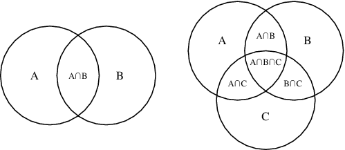
More to explore:
idempotents
orthogonal idempotents
Jacobson radical
Saturday, 30 April 2016
Find all $x\in \Bbb Z_{85}$ s.t. $(x+2)^{100}=0$.
Find all $x\in \Bbb Z_{85}$ s.t. $(x+2)^{100}=0$.
I: Taking Logarithm
Solving $(x+2)^{100}=0$ for $x\in \Bbb Z_{85}$ is equivalent to finding $x\in \Bbb Z_{85}$ s.t. $(x+2)^{100}=85y$. $$\begin{align}(x+2)^{100}&=85y\\ 100\log(x+2)&=\log(85y)\\ \log(x+2)&=\dfrac{\log(85y)}{100}\\ x+2&=10^{\log(85y)/100}\end{align}$$ The only integer values of $10^{\log(85y)/100}$ are $85,85^2,\cdots,$ (powers of $85$). [For example, when $y=85^{99}$, $10^{\log(85y)/100}=10^{\log(85)}=85$. When $y=85^{199}$, $10^{\log(85y)/100}=10^{2\log(85)}=85^2$.] It follows that $x=85-2,85^2-2,\cdots,$ (powers of $85$)$-2$. But all these values are equal to $-2\equiv_{85} 83$. Therefore, the only $x\in \Bbb Z_{85}$ satisfying the equation is $83$.
II: Solving System of Congruences
Solving $(x+2)^{100}=0$ for $x\in \Bbb Z_{85}$ is equivalent to solving $(x+2)^{100}\equiv_{85} 0$. Note that $85=5\cdot 17$. We can solve the following system of congruences: $$(x+2)^{100}\equiv_5 0\\ (x+2)^{100}\equiv_{17} 0.$$ Some calculations reveal that $$x\equiv_5 3\\ x\equiv_{17} 15.$$ Therefore, there exists $y\in \Bbb Z$ s.t. $x=3+5y$ and thus $$3+5y\equiv_{17} 15\\ 5y\equiv_{17} 12\\ y\equiv_{17} 12\cdot 7\\ y\equiv_{17} 16.$$ Finally, there exists $z\in \Bbb Z$ s.t. $x=3+5(16+17y)=83+85z\equiv_{85} 83$. Alternatively, by Chinese Remainder Theorem, the system has a unique solution $x$ modulo $85$. We have $$n_1=5,n_2=17;\;\;\;\text{and}\;\;\;n_1'=17,n_2'=5\\t_1=-2,t_2=7\\x=a_1t_1n_1'+a_2t_2n_2'=3\cdot -2\cdot 17+15\cdot 7\cdot 5=423\equiv_{85} 83.$$
I: Taking Logarithm
Solving $(x+2)^{100}=0$ for $x\in \Bbb Z_{85}$ is equivalent to finding $x\in \Bbb Z_{85}$ s.t. $(x+2)^{100}=85y$. $$\begin{align}(x+2)^{100}&=85y\\ 100\log(x+2)&=\log(85y)\\ \log(x+2)&=\dfrac{\log(85y)}{100}\\ x+2&=10^{\log(85y)/100}\end{align}$$ The only integer values of $10^{\log(85y)/100}$ are $85,85^2,\cdots,$ (powers of $85$). [For example, when $y=85^{99}$, $10^{\log(85y)/100}=10^{\log(85)}=85$. When $y=85^{199}$, $10^{\log(85y)/100}=10^{2\log(85)}=85^2$.] It follows that $x=85-2,85^2-2,\cdots,$ (powers of $85$)$-2$. But all these values are equal to $-2\equiv_{85} 83$. Therefore, the only $x\in \Bbb Z_{85}$ satisfying the equation is $83$.
II: Solving System of Congruences
Solving $(x+2)^{100}=0$ for $x\in \Bbb Z_{85}$ is equivalent to solving $(x+2)^{100}\equiv_{85} 0$. Note that $85=5\cdot 17$. We can solve the following system of congruences: $$(x+2)^{100}\equiv_5 0\\ (x+2)^{100}\equiv_{17} 0.$$ Some calculations reveal that $$x\equiv_5 3\\ x\equiv_{17} 15.$$ Therefore, there exists $y\in \Bbb Z$ s.t. $x=3+5y$ and thus $$3+5y\equiv_{17} 15\\ 5y\equiv_{17} 12\\ y\equiv_{17} 12\cdot 7\\ y\equiv_{17} 16.$$ Finally, there exists $z\in \Bbb Z$ s.t. $x=3+5(16+17y)=83+85z\equiv_{85} 83$. Alternatively, by Chinese Remainder Theorem, the system has a unique solution $x$ modulo $85$. We have $$n_1=5,n_2=17;\;\;\;\text{and}\;\;\;n_1'=17,n_2'=5\\t_1=-2,t_2=7\\x=a_1t_1n_1'+a_2t_2n_2'=3\cdot -2\cdot 17+15\cdot 7\cdot 5=423\equiv_{85} 83.$$
Friday, 29 April 2016
Dimension of Vector Space
Determine whether each of the following is a vector space and find the dimension and a basis for each that is a vector space:
i) $\mathbb{C}$ over $\mathbb{C}$.
ii) $\mathbb{C}$ over $\mathbb{R}$.
iii) $\mathbb{R}$ over $\mathbb{C}$.
iv) $\mathbb{R}$ over $\mathbb{Q}$.
v) $\mathbb{Q}$ over $\mathbb{R}$.
vi) $\mathbb{Q}$ over $\mathbb{Z}$.
vii) $\mathbb{S}=\{a+b\sqrt{2}+c\sqrt{5}\:|\:a,b,c \in \mathbb{Q}\}$ over $\mathbb{Q,R,\text{or}\: C}$.
Answers:
i) Yes. $\{1\}$ is a basis. Dimension is $1$.
[Say $1+2i,1+i\in \Bbb C$. $(1+2i)\cdot (1+i)=-1+3i=1\cdot (-1+3i)$, where $1$ is the basis element and $-1+3i$ is in the field $\Bbb C$.]
ii) Yes. $\{1,i\}$ is a basis. Dimension is $2$.
[Say $1+i\in \Bbb C$ and $2\in \Bbb R$. $2\cdot (1+i)=2+2i=2\cdot 1+2\cdot i$, where $1,i$ are elements in the basis and $2$ is in the field $\Bbb R$.]
iii) No. $i\in \Bbb C$ and $1\in \Bbb R$, but $i \cdot 1=i\notin \Bbb R$.
iv) Yes. $\{1,\pi,\pi^2,\cdots\}$ are linearly independent over $\Bbb Q$. Dimension is infinite.
v) No. $\sqrt{2}\in \Bbb R$ and $1\in \Bbb Q$, but $\sqrt{2} \cdot 1=\sqrt{2}\notin \Bbb Q$.
vi) No. $\Bbb Z$ is not a field.
vii) Yes only over $\Bbb Q$. $\{1,\sqrt{2},\sqrt{5}\}$ is a basis. Dimension is $3$.
From iii and v, we know that the field is always 'smaller' than its vector space. In fact, this is related to the concept of field extension (to be discussed in our next post).
Let $V=\{(x,y)\:|\:x,y\in \Bbb C\}$. Under the standard addition and scalar multiplication for ordered pairs of complex numbers, is $V$ a vector space over $\Bbb C$? Over $\Bbb R$? Over $\Bbb Q$? If so, find the dimension of $V$.
Answers:
From the previous question, we know $\{(1,0),(0,1)\}$ form a basis for $V$ over $\Bbb C$. Dimension is $2$. $\{(1,0),(i,0),(0,1),(0,i)\}$ form a basis for $V$ over $\Bbb R$. Dimension is $4$. Lastly, the dimension of $V$ over $\Bbb Q$ is infinite.
i) $\mathbb{C}$ over $\mathbb{C}$.
ii) $\mathbb{C}$ over $\mathbb{R}$.
iii) $\mathbb{R}$ over $\mathbb{C}$.
iv) $\mathbb{R}$ over $\mathbb{Q}$.
v) $\mathbb{Q}$ over $\mathbb{R}$.
vi) $\mathbb{Q}$ over $\mathbb{Z}$.
vii) $\mathbb{S}=\{a+b\sqrt{2}+c\sqrt{5}\:|\:a,b,c \in \mathbb{Q}\}$ over $\mathbb{Q,R,\text{or}\: C}$.
Answers:
i) Yes. $\{1\}$ is a basis. Dimension is $1$.
[Say $1+2i,1+i\in \Bbb C$. $(1+2i)\cdot (1+i)=-1+3i=1\cdot (-1+3i)$, where $1$ is the basis element and $-1+3i$ is in the field $\Bbb C$.]
ii) Yes. $\{1,i\}$ is a basis. Dimension is $2$.
[Say $1+i\in \Bbb C$ and $2\in \Bbb R$. $2\cdot (1+i)=2+2i=2\cdot 1+2\cdot i$, where $1,i$ are elements in the basis and $2$ is in the field $\Bbb R$.]
iii) No. $i\in \Bbb C$ and $1\in \Bbb R$, but $i \cdot 1=i\notin \Bbb R$.
iv) Yes. $\{1,\pi,\pi^2,\cdots\}$ are linearly independent over $\Bbb Q$. Dimension is infinite.
v) No. $\sqrt{2}\in \Bbb R$ and $1\in \Bbb Q$, but $\sqrt{2} \cdot 1=\sqrt{2}\notin \Bbb Q$.
vi) No. $\Bbb Z$ is not a field.
vii) Yes only over $\Bbb Q$. $\{1,\sqrt{2},\sqrt{5}\}$ is a basis. Dimension is $3$.
From iii and v, we know that the field is always 'smaller' than its vector space. In fact, this is related to the concept of field extension (to be discussed in our next post).
Let $V=\{(x,y)\:|\:x,y\in \Bbb C\}$. Under the standard addition and scalar multiplication for ordered pairs of complex numbers, is $V$ a vector space over $\Bbb C$? Over $\Bbb R$? Over $\Bbb Q$? If so, find the dimension of $V$.
Answers:
From the previous question, we know $\{(1,0),(0,1)\}$ form a basis for $V$ over $\Bbb C$. Dimension is $2$. $\{(1,0),(i,0),(0,1),(0,i)\}$ form a basis for $V$ over $\Bbb R$. Dimension is $4$. Lastly, the dimension of $V$ over $\Bbb Q$ is infinite.
Saturday, 23 April 2016
A problem on diagonalisation
Give examples of the following types of operators defined by a $2\times 2$ matrix or explain why such an operator can't exist:
i) diagonalisable, invertible,
ii) diagonalisable, not invertible,
iii) not diagonalisable, invertible,
iv) not diagonalisable, not invertible.
Let's just consider the case in $\Bbb R$.
i) $$\boxed{\begin{pmatrix}a&0\\0&b\end{pmatrix},\quad \text{a and b are not necessarily different},\quad a,b\neq 0}$$ Any diagonal matrix $D$ is diagonalisable: $$I_n DI_n=D.\\ \boxed{\begin{pmatrix}a&b\\b&a\end{pmatrix},\quad a\neq b,\quad a\neq -b,\quad\text{a can be zero.}}$$ Calculations: $(a-\lambda)^2-b^2=0\Rightarrow \lambda=a-b,a+b$. $$\ker\begin{pmatrix}a-(a+b)&b\\b&a-(a+b)\end{pmatrix}=\text{span}\bigg\{\begin{pmatrix}1\\1\end{pmatrix}\bigg\}\\ \ker\begin{pmatrix}a-(a-b)&b\\b&a-(a-b)\end{pmatrix}=\text{span}\bigg\{\begin{pmatrix}1\\-1\end{pmatrix}\bigg\}$$ The two eigenvectors form an eigenbasis. Alternatively, one can use the result: if $A\in M_{n\times n}(\Bbb F)$ has $n$ distinct eigenvalues in $\Bbb F$, then $A$ is diagonalisable over $\Bbb F$. $$\boxed{\begin{pmatrix}a&b\\b&c\end{pmatrix},\quad a\neq c,\quad b\neq 0,\quad\text{a can be zero.}}$$ The calculation is similar, but involves the use of quadratic formula. Since $a\neq c$ and $b\neq 0$, we have two distinct eigenvalues. Symmetric matrices are thus diagonalisable. $$\boxed{\begin{pmatrix}a&b\\0&c\end{pmatrix},\quad a\neq c,\quad b\neq 0}$$ Upper triangular matrices with distinct diagonal entries are diagonalisable because of the same reason: they have distinct eigenvalues. The above matrices are invertible since their determinants are non-zero.
ii) $$\boxed{\begin{pmatrix}a&0\\0&0\end{pmatrix},\quad a\neq 0}$$ Again, any diagonal matrix is diagonalisable. $$\boxed{\begin{pmatrix}a&a\\a&a\end{pmatrix},\quad a\neq 0}$$ Calculation: $(a-\lambda)^2-a^2=0\Rightarrow \lambda=0,2a$. When $a=1$, the matrix is called matrix of ones. $$\boxed{\begin{pmatrix}a&a\\b&b\end{pmatrix}, \begin{pmatrix}a&b\\a&b\end{pmatrix},\quad a+b\neq 0,\;\;\text{a,b not both zero.}}$$Calculation: $(a-\lambda)(b-\lambda)-ab=0\Rightarrow \lambda=0,a+b$.
iii) $$\boxed{\begin{pmatrix}a&b\\0&a\end{pmatrix},\begin{pmatrix}a&0\\b&a\end{pmatrix},\quad \text{a and b are not necessarily different},\quad a,b\neq 0}$$ These are known as the shear transformations, which are not diagonalisable. Proof by contradiction: Suppose $\begin{pmatrix}a&b\\0&a\end{pmatrix}$ is diagonalisable. Then there exist a diagonal matrix $D$ and an invertible matrix $V$ s.t. $$\begin{pmatrix}a&b\\0&a\end{pmatrix}=V^{-1}DV.$$ We know just by looking at the matrix that $a$ is an eigenvalue with multiplicity $2$. So $D=\begin{pmatrix}a&0\\0&a\end{pmatrix}=aI_2$. We then have $\begin{pmatrix}a&b\\0&a\end{pmatrix}=aV^{-1}I_2V=aI_2=\begin{pmatrix}a&0\\0&a\end{pmatrix}$ which is a contradiction.
iv) $$\boxed{\begin{pmatrix}0&a\\0&0\end{pmatrix},\quad a\neq 0}$$ Its only eigenvalue is $0$ of multiplicity $2$.
From this problem, we see that invertibility does not necessarily nor sufficiently imply diagonalisability! Another important fact that one can observe from (ii) and (iv) is that if a square matrix $A$ is not invertible, then $\lambda=0$ is an eigenvalue of $A$. The converse also holds: if $\lambda=0$ is an eigenvalue of $A$, then $A$ is not invertible.
Claim: $A\in M_{n\times n}(\Bbb F)$ is singular iff $\lambda=0$ is an eigenvalue of $A$.
Proof: $\lambda=0$ is a solution of the characteristic equation $\lambda^n+c_1\lambda^{n-1}+\cdots+c_n=0$ iff $c_n=0$. By definition, $\det(\lambda I-A)=\lambda^n+c_1\lambda^{n-1}+\cdots+c_n$. When $\lambda=0$, we have $\det(\lambda I-A)=\det(-A)=(-1)^n\det(A)=c_n$. We thus have $\det(A)=0$ iff $c_n=0$ iff $\lambda=0.\;\Box$
Here's a summary:
i) diagonalisable, invertible: symmetric, upper triangular, diagonal
ii) diagonalisable, not invertible: nilpotent, scalar multiples of matrix of ones
iii) not diagonalisable, invertible: shear
iv) not diagonalisable, not invertible: nilpotent.
I tried to enumerate all possibilities but failed. I can't imagine the amount of work it takes to characterise diagonalisation for $3\times 3$ matrices...
Questions:
$$\boxed{\begin{pmatrix}a&b\\c&d\end{pmatrix},\quad (a-d)^2=-4bc,\quad ad-bc\neq 0}$$ has repeated eigenvalues, so I consider it fitting (iii), but can the kernel corresponding to that one eigenvalue be spanned by two eigenvectors? Similar questions for $$\boxed{\begin{pmatrix}a&a\\a&b\end{pmatrix},\quad 5a^2+b^2=2ab,\quad a(b-a)\neq 0}\\
\boxed{\begin{pmatrix}a&a\\b&c\end{pmatrix},\quad a^2+c^2=2ac-4ab,\quad a(c-b)\neq 0}\\
\boxed{\begin{pmatrix}0&a\\b&c\end{pmatrix},\quad c^2=-4ab,\quad ab\neq 0}$$ I'm not even sure if there are other possibilities for (iii) and (iv).
i) diagonalisable, invertible,
ii) diagonalisable, not invertible,
iii) not diagonalisable, invertible,
iv) not diagonalisable, not invertible.
Let's just consider the case in $\Bbb R$.
i) $$\boxed{\begin{pmatrix}a&0\\0&b\end{pmatrix},\quad \text{a and b are not necessarily different},\quad a,b\neq 0}$$ Any diagonal matrix $D$ is diagonalisable: $$I_n DI_n=D.\\ \boxed{\begin{pmatrix}a&b\\b&a\end{pmatrix},\quad a\neq b,\quad a\neq -b,\quad\text{a can be zero.}}$$ Calculations: $(a-\lambda)^2-b^2=0\Rightarrow \lambda=a-b,a+b$. $$\ker\begin{pmatrix}a-(a+b)&b\\b&a-(a+b)\end{pmatrix}=\text{span}\bigg\{\begin{pmatrix}1\\1\end{pmatrix}\bigg\}\\ \ker\begin{pmatrix}a-(a-b)&b\\b&a-(a-b)\end{pmatrix}=\text{span}\bigg\{\begin{pmatrix}1\\-1\end{pmatrix}\bigg\}$$ The two eigenvectors form an eigenbasis. Alternatively, one can use the result: if $A\in M_{n\times n}(\Bbb F)$ has $n$ distinct eigenvalues in $\Bbb F$, then $A$ is diagonalisable over $\Bbb F$. $$\boxed{\begin{pmatrix}a&b\\b&c\end{pmatrix},\quad a\neq c,\quad b\neq 0,\quad\text{a can be zero.}}$$ The calculation is similar, but involves the use of quadratic formula. Since $a\neq c$ and $b\neq 0$, we have two distinct eigenvalues. Symmetric matrices are thus diagonalisable. $$\boxed{\begin{pmatrix}a&b\\0&c\end{pmatrix},\quad a\neq c,\quad b\neq 0}$$ Upper triangular matrices with distinct diagonal entries are diagonalisable because of the same reason: they have distinct eigenvalues. The above matrices are invertible since their determinants are non-zero.
ii) $$\boxed{\begin{pmatrix}a&0\\0&0\end{pmatrix},\quad a\neq 0}$$ Again, any diagonal matrix is diagonalisable. $$\boxed{\begin{pmatrix}a&a\\a&a\end{pmatrix},\quad a\neq 0}$$ Calculation: $(a-\lambda)^2-a^2=0\Rightarrow \lambda=0,2a$. When $a=1$, the matrix is called matrix of ones. $$\boxed{\begin{pmatrix}a&a\\b&b\end{pmatrix}, \begin{pmatrix}a&b\\a&b\end{pmatrix},\quad a+b\neq 0,\;\;\text{a,b not both zero.}}$$Calculation: $(a-\lambda)(b-\lambda)-ab=0\Rightarrow \lambda=0,a+b$.
iii) $$\boxed{\begin{pmatrix}a&b\\0&a\end{pmatrix},\begin{pmatrix}a&0\\b&a\end{pmatrix},\quad \text{a and b are not necessarily different},\quad a,b\neq 0}$$ These are known as the shear transformations, which are not diagonalisable. Proof by contradiction: Suppose $\begin{pmatrix}a&b\\0&a\end{pmatrix}$ is diagonalisable. Then there exist a diagonal matrix $D$ and an invertible matrix $V$ s.t. $$\begin{pmatrix}a&b\\0&a\end{pmatrix}=V^{-1}DV.$$ We know just by looking at the matrix that $a$ is an eigenvalue with multiplicity $2$. So $D=\begin{pmatrix}a&0\\0&a\end{pmatrix}=aI_2$. We then have $\begin{pmatrix}a&b\\0&a\end{pmatrix}=aV^{-1}I_2V=aI_2=\begin{pmatrix}a&0\\0&a\end{pmatrix}$ which is a contradiction.
iv) $$\boxed{\begin{pmatrix}0&a\\0&0\end{pmatrix},\quad a\neq 0}$$ Its only eigenvalue is $0$ of multiplicity $2$.
From this problem, we see that invertibility does not necessarily nor sufficiently imply diagonalisability! Another important fact that one can observe from (ii) and (iv) is that if a square matrix $A$ is not invertible, then $\lambda=0$ is an eigenvalue of $A$. The converse also holds: if $\lambda=0$ is an eigenvalue of $A$, then $A$ is not invertible.
Claim: $A\in M_{n\times n}(\Bbb F)$ is singular iff $\lambda=0$ is an eigenvalue of $A$.
Proof: $\lambda=0$ is a solution of the characteristic equation $\lambda^n+c_1\lambda^{n-1}+\cdots+c_n=0$ iff $c_n=0$. By definition, $\det(\lambda I-A)=\lambda^n+c_1\lambda^{n-1}+\cdots+c_n$. When $\lambda=0$, we have $\det(\lambda I-A)=\det(-A)=(-1)^n\det(A)=c_n$. We thus have $\det(A)=0$ iff $c_n=0$ iff $\lambda=0.\;\Box$
Here's a summary:
i) diagonalisable, invertible: symmetric, upper triangular, diagonal
ii) diagonalisable, not invertible: nilpotent, scalar multiples of matrix of ones
iii) not diagonalisable, invertible: shear
iv) not diagonalisable, not invertible: nilpotent.
I tried to enumerate all possibilities but failed. I can't imagine the amount of work it takes to characterise diagonalisation for $3\times 3$ matrices...
Questions:
$$\boxed{\begin{pmatrix}a&b\\c&d\end{pmatrix},\quad (a-d)^2=-4bc,\quad ad-bc\neq 0}$$ has repeated eigenvalues, so I consider it fitting (iii), but can the kernel corresponding to that one eigenvalue be spanned by two eigenvectors? Similar questions for $$\boxed{\begin{pmatrix}a&a\\a&b\end{pmatrix},\quad 5a^2+b^2=2ab,\quad a(b-a)\neq 0}\\
\boxed{\begin{pmatrix}a&a\\b&c\end{pmatrix},\quad a^2+c^2=2ac-4ab,\quad a(c-b)\neq 0}\\
\boxed{\begin{pmatrix}0&a\\b&c\end{pmatrix},\quad c^2=-4ab,\quad ab\neq 0}$$ I'm not even sure if there are other possibilities for (iii) and (iv).
Tuesday, 19 April 2016
Evaluate $\lim_n \dfrac{\sqrt[n]{n!}}{n}$
Prove that $$\lim_{n\to \infty} \dfrac{\sqrt[n]{n!}}{n}=e^{-1}.$$
I: Taking logarithm
Since $\ln \dfrac{\sqrt[n]{n!}}{n}=\ln \sqrt[n]{\dfrac{n!}{n^n}}=\dfrac{1}{n}\bigg(\ln \dfrac{1}{n}+\ln \dfrac{2}{n}+\cdots+\ln \dfrac{n}{n}\bigg)$, we have $$\begin{align}\lim_{n\to \infty} \dfrac{\sqrt[n]{n!}}{n} &=\exp\bigg(\lim\limits_{n\to \infty}(\dfrac{1}{n}\sum\limits_{k=1}^n\ln \dfrac{k}{n})\bigg)\\ &=\exp\bigg(\int_0^1 \ln x\;dx\bigg)\\ &=e^{-1}\;\Box\end{align}$$
II: Sandwich theorem
For any sequence $(a_n)$ of positive real numbers, we have $$\liminf_n \dfrac{a_{n+1}}{a_n}\leq \liminf_n a_n^{1/n}\leq \limsup_n a_n^{1/n}\leq \limsup_n \dfrac{a_{n+1}}{a_n}$$ Pick $a_n=\dfrac{n!}{n^n}$. Then $\dfrac{a_{n+1}}{a_n}=(1+\dfrac{1}{n})^{-n}$ and $a_n^{1/n}=\dfrac{\sqrt[n]{n!}}{n}$. It follows that $$\liminf_n (1+\dfrac{1}{n})^{-n}\leq \liminf_n \dfrac{\sqrt[n]{n!}}{n}\leq \limsup_n \dfrac{\sqrt[n]{n!}}{n}\leq \limsup_n (1+\dfrac{1}{n})^{-n}.$$ We know $$\liminf_n (1+\dfrac{1}{n})^{-n}=\limsup_n (1+\dfrac{1}{n})^{-n}=e^{-1}.$$ By sandwich theorem, we have $$\liminf_n \dfrac{\sqrt[n]{n!}}{n}=\limsup_n \dfrac{\sqrt[n]{n!}}{n}=\lim_n \dfrac{\sqrt[n]{n!}}{n}=e^{-1}\;\Box$$
III: Stirling approximation $$n!\sim \sqrt{2\pi n}(\dfrac{n}{e})^n\\ \dfrac{\sqrt[n]{n!}}{n}\sim \dfrac{\sqrt[2n]{2\pi}e^{-1}n^{1+1/(2n)}}{n}\to e^{-1}\;\Box$$
IV: Lemma: If $\lim_{n\to\infty}a_n=a$ and $a_n>0$ for all $n$, then we have $$ \lim_{n\to\infty}\sqrt[n]{a_1a_2\cdots a_n}=a.$$ Pick $a_n=\bigg(1+\dfrac{1}{n}\bigg)^n$. Since $a_n>0$ for all $n$ and $\lim_{n\to \infty}a_n=e$, we can apply the lemma: $$\begin{align} e&=\lim_{n\to\infty}\sqrt[n]{a_1a_2\cdots a_n}\\ &=\lim_{n\to\infty}\sqrt[n]{\left(\frac{2}{1}\right)^1\left(\frac{3}{2}\right)^2\cdots\left(\frac{n+1}{n}\right)^n}\\ &=\lim_{n\to\infty}\sqrt[n]{\frac{(n+1)^n}{n!}}\\&= \lim_{n\to\infty}\frac{n+1}{\sqrt[n]{n!}}\\&=\lim_{n\to\infty}\frac{n}{\sqrt[n]{n!}}+\lim_{n\to\infty}\frac{1}{\sqrt[n]{n!}} \tag{*}\\&=\lim_{n\to\infty}\frac{n}{\sqrt[n]{n!}},\end{align}$$ where in $(*)$ we have also used the lemma for $a_n=\dfrac{1}{n}\to 0$. It follows that $$\lim_{n\to \infty} \dfrac{\sqrt[n]{n!}}{n}=e^{-1}\;\Box$$
Reference
mse
I: Taking logarithm
Since $\ln \dfrac{\sqrt[n]{n!}}{n}=\ln \sqrt[n]{\dfrac{n!}{n^n}}=\dfrac{1}{n}\bigg(\ln \dfrac{1}{n}+\ln \dfrac{2}{n}+\cdots+\ln \dfrac{n}{n}\bigg)$, we have $$\begin{align}\lim_{n\to \infty} \dfrac{\sqrt[n]{n!}}{n} &=\exp\bigg(\lim\limits_{n\to \infty}(\dfrac{1}{n}\sum\limits_{k=1}^n\ln \dfrac{k}{n})\bigg)\\ &=\exp\bigg(\int_0^1 \ln x\;dx\bigg)\\ &=e^{-1}\;\Box\end{align}$$
II: Sandwich theorem
For any sequence $(a_n)$ of positive real numbers, we have $$\liminf_n \dfrac{a_{n+1}}{a_n}\leq \liminf_n a_n^{1/n}\leq \limsup_n a_n^{1/n}\leq \limsup_n \dfrac{a_{n+1}}{a_n}$$ Pick $a_n=\dfrac{n!}{n^n}$. Then $\dfrac{a_{n+1}}{a_n}=(1+\dfrac{1}{n})^{-n}$ and $a_n^{1/n}=\dfrac{\sqrt[n]{n!}}{n}$. It follows that $$\liminf_n (1+\dfrac{1}{n})^{-n}\leq \liminf_n \dfrac{\sqrt[n]{n!}}{n}\leq \limsup_n \dfrac{\sqrt[n]{n!}}{n}\leq \limsup_n (1+\dfrac{1}{n})^{-n}.$$ We know $$\liminf_n (1+\dfrac{1}{n})^{-n}=\limsup_n (1+\dfrac{1}{n})^{-n}=e^{-1}.$$ By sandwich theorem, we have $$\liminf_n \dfrac{\sqrt[n]{n!}}{n}=\limsup_n \dfrac{\sqrt[n]{n!}}{n}=\lim_n \dfrac{\sqrt[n]{n!}}{n}=e^{-1}\;\Box$$
III: Stirling approximation $$n!\sim \sqrt{2\pi n}(\dfrac{n}{e})^n\\ \dfrac{\sqrt[n]{n!}}{n}\sim \dfrac{\sqrt[2n]{2\pi}e^{-1}n^{1+1/(2n)}}{n}\to e^{-1}\;\Box$$
IV: Lemma: If $\lim_{n\to\infty}a_n=a$ and $a_n>0$ for all $n$, then we have $$ \lim_{n\to\infty}\sqrt[n]{a_1a_2\cdots a_n}=a.$$ Pick $a_n=\bigg(1+\dfrac{1}{n}\bigg)^n$. Since $a_n>0$ for all $n$ and $\lim_{n\to \infty}a_n=e$, we can apply the lemma: $$\begin{align} e&=\lim_{n\to\infty}\sqrt[n]{a_1a_2\cdots a_n}\\ &=\lim_{n\to\infty}\sqrt[n]{\left(\frac{2}{1}\right)^1\left(\frac{3}{2}\right)^2\cdots\left(\frac{n+1}{n}\right)^n}\\ &=\lim_{n\to\infty}\sqrt[n]{\frac{(n+1)^n}{n!}}\\&= \lim_{n\to\infty}\frac{n+1}{\sqrt[n]{n!}}\\&=\lim_{n\to\infty}\frac{n}{\sqrt[n]{n!}}+\lim_{n\to\infty}\frac{1}{\sqrt[n]{n!}} \tag{*}\\&=\lim_{n\to\infty}\frac{n}{\sqrt[n]{n!}},\end{align}$$ where in $(*)$ we have also used the lemma for $a_n=\dfrac{1}{n}\to 0$. It follows that $$\lim_{n\to \infty} \dfrac{\sqrt[n]{n!}}{n}=e^{-1}\;\Box$$
Reference
mse
Saturday, 2 April 2016
Primitive Roots, Discrete Logarithms
(a) Show that for each element $x\in \Bbb Z_{19}^\times$ there is a number $n\in \Bbb N$ s.t. $x=[2]^n.$
(b) Show that the function $$\log:\begin{align}\Bbb Z_{19}^\times&\to \Bbb Z_{18}\\ [2]^n&\mapsto n\end{align}$$ is well-defined and has the property that $\log(xy)=\log x+\log y,\log(x/y)=\log x-\log y$ and $\log x^r=r\log x$ for all $x,y\in \Bbb Z_{19}^\times$ and all $r\in \Bbb Z$.
(c) List the values of this function and use them to determine $30^{14}\;\text{mod}\;19$ and $25^{11}\;\text{mod}\;19$.
Food for thought:
Intuition for (a)? Is it related to period?
Why choose $2$ in particular? Will other numbers work? [Yes! Read till the end.]
Any applications in modular exponentiation? [Yes, discrete logarithms are used in cryptography!]
I only worked on (a) and (c).
(a) My failed attempts: I expressed $x$ as $x=2^n+19y\;\exists\; y\in \Bbb Z$ and tried to use the fact that $(2,19)=1$, which didn't work. The next day I thought of proving $$\log:\begin{align}\Bbb Z_{19}^\times&\to \Bbb Z_{18}\\ [2]^n&\mapsto n\end{align}$$ is surjective, but I can't find $n$ in terms of $x$ explicitly. A simple proof is to prove that $\Bbb Z_{19}$ is a cyclic group with generator $2$, which follows from the results in (c).
This problem is actually related to primitive roots. If $a$ is a primitive root modulo $n$, then every element of $\Bbb Z_n$ is a power of $a$. Or in the language of group theory: $a$ is a primitive root modulo $n$ if $a$ is a generator of the multiplicative group on non-zero objects modulo $n$. Here we state without proof a handy result for proving (a): $a$ is a primitive root modulo $p$ if it has order $p-1$. [To be proved later]
Recall Fermat's little theorem: if $p$ is a prime, $x\in \Bbb Z$ and $p\not\mid a$, then $a^{p-1}\equiv_p 1$. Recall also the definition of order of $a$ modulo $n$, $\text{ord}_n a$, for positive integer $n>1$ and integer $x$, if there exists a least positive integer $k$ s.t. $a^k\equiv_n 1$, then $\text{ord}_n a=k$ is the order. When we have $\text{ord}_p a=p-1$, $a$ is a primitive root modulo $p$.
Therefore, to prove (a), we need to prove that $2$ is a primitive root modulo $19$, which is true because $2^{18}\equiv_{19}1$.
(c) I used matlab to generate powers of two modulo 19.
'Logarithm table' form:
n: 0 1 2 3 4 5 6 7 8 9 10 11 12 13 14 15 16 17
log(2^n): 1 2 4 8 16 13 7 14 9 18 17 15 11 3 6 12 5 10
We now find $30^{14}\;\text{mod}\;19$ and $25^{11}\;\text{mod}\;19$: $$\begin{align}30^{14}&\equiv_{19}2^{14}\;15^{14}\\
&\equiv_{19}2^{14}\;34^{14}\\
&\equiv_{19}2^{14}\;2^{14}\;17^{14}\\
&\equiv_{19}2^{14}\;2^{14}\;(-2)^{14}\\
&\equiv_{19}2^{6}\quad \qquad [2^{18}=1]\\
&\equiv_{19}7\;\;\Box
\end{align}$$
$$\begin{align}25^{11}&\equiv_{19}6^{11}\\
&\equiv_{19}2^{11}\;3^{11}\\
&\equiv_{19}2^{11}\;22^{11}\\
&\equiv_{19}2^{11}\;2^{11}\;(-8)^{11}\\
&\equiv_{19}2^4\;(-2^{33})\\
&\equiv_{19}-2\\
&\equiv_{19}17\;\;\Box
\end{align}$$
Lessons learnt:
At first I thought $[2]^n\mapsto n$ means $n$ is one value, namely, $[2]^1\mapsto 1$, but later I realised it doesn't make sense! The values of the range are just the values of $2^n\;\text{mod}\;19$, which are $1,2,3,\cdots,18$. This makes sense because there are $\phi(19)=19-1=18$ elements in $\Bbb Z_{19}^\times$, which explains why the range is $\Bbb Z_{18}$.
Also, I should rely on my brain rather than matlab: $\text{mod}(30^{14},19)$ in matlab gives $0$ but the answer is really $7$. ($\text{mod}(11^{14},19)$ in matlab gives $7$ though...)
Extensions:
Replacing $2$ by $3$ works.
$$\log:\begin{align}\Bbb Z_{19}^\times&\to \Bbb Z_{18}\\ [3]^n&\mapsto n\end{align}\\ 30^{14}\equiv_{19}3^{14}\;(-3)^{28}\equiv_{19}3^6\equiv_{19}7\\ 25^{11}\equiv_{19}6^{11}\equiv_{19}2^{11}3^{11}\equiv_{19}15\cdot 10\equiv_{19}17$$ In fact, $10,13,14,15$ also work because they are also primitive roots. (Question: How to find all primitive roots modulo a number?)
More to learn:
cryptography
an advanced proof that $\Bbb Z_p^\times \cong \Bbb Z_{p-1}$
cyclicity of $\Bbb Z_p^\times$
using primitive roots to solve problems
(b) Show that the function $$\log:\begin{align}\Bbb Z_{19}^\times&\to \Bbb Z_{18}\\ [2]^n&\mapsto n\end{align}$$ is well-defined and has the property that $\log(xy)=\log x+\log y,\log(x/y)=\log x-\log y$ and $\log x^r=r\log x$ for all $x,y\in \Bbb Z_{19}^\times$ and all $r\in \Bbb Z$.
(c) List the values of this function and use them to determine $30^{14}\;\text{mod}\;19$ and $25^{11}\;\text{mod}\;19$.
Food for thought:
Intuition for (a)? Is it related to period?
Why choose $2$ in particular? Will other numbers work? [Yes! Read till the end.]
Any applications in modular exponentiation? [Yes, discrete logarithms are used in cryptography!]
I only worked on (a) and (c).
(a) My failed attempts: I expressed $x$ as $x=2^n+19y\;\exists\; y\in \Bbb Z$ and tried to use the fact that $(2,19)=1$, which didn't work. The next day I thought of proving $$\log:\begin{align}\Bbb Z_{19}^\times&\to \Bbb Z_{18}\\ [2]^n&\mapsto n\end{align}$$ is surjective, but I can't find $n$ in terms of $x$ explicitly. A simple proof is to prove that $\Bbb Z_{19}$ is a cyclic group with generator $2$, which follows from the results in (c).
This problem is actually related to primitive roots. If $a$ is a primitive root modulo $n$, then every element of $\Bbb Z_n$ is a power of $a$. Or in the language of group theory: $a$ is a primitive root modulo $n$ if $a$ is a generator of the multiplicative group on non-zero objects modulo $n$. Here we state without proof a handy result for proving (a): $a$ is a primitive root modulo $p$ if it has order $p-1$. [To be proved later]
Recall Fermat's little theorem: if $p$ is a prime, $x\in \Bbb Z$ and $p\not\mid a$, then $a^{p-1}\equiv_p 1$. Recall also the definition of order of $a$ modulo $n$, $\text{ord}_n a$, for positive integer $n>1$ and integer $x$, if there exists a least positive integer $k$ s.t. $a^k\equiv_n 1$, then $\text{ord}_n a=k$ is the order. When we have $\text{ord}_p a=p-1$, $a$ is a primitive root modulo $p$.
Therefore, to prove (a), we need to prove that $2$ is a primitive root modulo $19$, which is true because $2^{18}\equiv_{19}1$.
| 2^0 = 1 (mod 19) 2^1 = 2 (mod 19) 2^2 = 4 (mod 19) 2^3 = 8 (mod 19) 2^4 = 16 (mod 19) 2^5 = 13 (mod 19) 2^6 = 7 (mod 19) | 2^7 = 14 (mod 19) 2^8 = 9 (mod 19) 2^9 = 18 (mod 19) 2^10 = 17 (mod 19) 2^11 = 15 (mod 19) 2^12 = 11 (mod 19) 2^13 = 3 (mod 19) | 2^14 = 6 (mod 19) 2^15 = 12 (mod 19) 2^16 = 5 (mod 19) 2^17 = 10 (mod 19) 2^18 = 1 (mod 19) 2^19 = 2 (mod 19) 2^20 = 4 (mod 19) |
'Logarithm table' form:
n: 0 1 2 3 4 5 6 7 8 9 10 11 12 13 14 15 16 17
log(2^n): 1 2 4 8 16 13 7 14 9 18 17 15 11 3 6 12 5 10
We now find $30^{14}\;\text{mod}\;19$ and $25^{11}\;\text{mod}\;19$: $$\begin{align}30^{14}&\equiv_{19}2^{14}\;15^{14}\\
&\equiv_{19}2^{14}\;34^{14}\\
&\equiv_{19}2^{14}\;2^{14}\;17^{14}\\
&\equiv_{19}2^{14}\;2^{14}\;(-2)^{14}\\
&\equiv_{19}2^{6}\quad \qquad [2^{18}=1]\\
&\equiv_{19}7\;\;\Box
\end{align}$$
$$\begin{align}25^{11}&\equiv_{19}6^{11}\\
&\equiv_{19}2^{11}\;3^{11}\\
&\equiv_{19}2^{11}\;22^{11}\\
&\equiv_{19}2^{11}\;2^{11}\;(-8)^{11}\\
&\equiv_{19}2^4\;(-2^{33})\\
&\equiv_{19}-2\\
&\equiv_{19}17\;\;\Box
\end{align}$$
Lessons learnt:
At first I thought $[2]^n\mapsto n$ means $n$ is one value, namely, $[2]^1\mapsto 1$, but later I realised it doesn't make sense! The values of the range are just the values of $2^n\;\text{mod}\;19$, which are $1,2,3,\cdots,18$. This makes sense because there are $\phi(19)=19-1=18$ elements in $\Bbb Z_{19}^\times$, which explains why the range is $\Bbb Z_{18}$.
Also, I should rely on my brain rather than matlab: $\text{mod}(30^{14},19)$ in matlab gives $0$ but the answer is really $7$. ($\text{mod}(11^{14},19)$ in matlab gives $7$ though...)
Extensions:
| 3^0 = 1 (mod 19) 3^1 = 3 (mod 19) 3^2 = 9 (mod 19) 3^3 = 8 (mod 19) 3^4 = 5 (mod 19) 3^5 = 15 (mod 19) 3^6 = 7 (mod 19) | 3^7 = 2 (mod 19) 3^8 = 6 (mod 19) 3^9 = 18 (mod 19) 3^10 = 16 (mod 19) 3^11 = 10 (mod 19) 3^12 = 11 (mod 19) 3^13 = 14 (mod 19) | 3^14 = 4 (mod 19) 3^15 = 12 (mod 19) 3^16 = 17 (mod 19) 3^17 = 13 (mod 19) 3^18 = 1 (mod 19) 3^19 = 3 (mod 19) 3^20 = 9 (mod 19) |
Replacing $2$ by $3$ works.
$$\log:\begin{align}\Bbb Z_{19}^\times&\to \Bbb Z_{18}\\ [3]^n&\mapsto n\end{align}\\ 30^{14}\equiv_{19}3^{14}\;(-3)^{28}\equiv_{19}3^6\equiv_{19}7\\ 25^{11}\equiv_{19}6^{11}\equiv_{19}2^{11}3^{11}\equiv_{19}15\cdot 10\equiv_{19}17$$ In fact, $10,13,14,15$ also work because they are also primitive roots. (Question: How to find all primitive roots modulo a number?)
More to learn:
cryptography
an advanced proof that $\Bbb Z_p^\times \cong \Bbb Z_{p-1}$
cyclicity of $\Bbb Z_p^\times$
using primitive roots to solve problems
Monday, 21 March 2016
Several inequalities
Let $m,n\in \Bbb N, x\in \Bbb R, x\geq 0, x\neq 1$. Prove the followings: if $m>n$, then $\dfrac{x^m-1}{m}>\dfrac{x^n-1}{n}$; if $m<n$, then $\dfrac{x^m-1}{m}<\dfrac{x^n-1}{n}$.
Proof:
Consider the case when $m>n$. The other case is similar. It suffices to show that $n(x^m-1)-m(x^n-1)> 0$ for $x>1$. $$\begin{align}n(x^m-1)-m(x^n-1)&=n(x-1)(x^{m-1}+x^{m-2}+\cdots+1)-m(x-1)(x^{n-1}+x^{n-2}+\cdots+1)\\&=n(x-1)(x^{m-1}+x^{m-2}+\cdots+x^n)+n(x-1)(x^{n-1}+x^{n-2}+\cdots+1)\\&\quad-m(x-1)(x^{n-1}+x^{n-2}+\cdots+1)\\&=n(x-1)(x^{m-1}+x^{m-2}+\cdots+x^n)\\&\quad-(m-n)(x-1)(x^{n-1}+x^{n-2}+\cdots+1)\\&> (x-1)[n\underbrace{(x^n+\cdots+x^n)}_{m-n\; terms}-(m-n)\underbrace{(x^n+\cdots+x^n)}_{n\; terms}]\qquad(*)\\&=(x-1)x^n[n(m-n)-(m-n)n]\\&=0\qquad \Box\end{align}$$ In $(*)$, we have used the facts that $x^{m-i}\geq x^n$ when $i=1,\cdots,m-n$ and $-x^{n-j}\geq -x^n$ where $j=1,\cdots,n$. The case for $0\leq x<1$ also holds because we have $-x^{m-i}\geq -x^n$ when $i=1,\cdots,m-n$ and $-x^{n-j}\leq -x^n$ where $j=1,\cdots,n$.
Remark: This result implies that the sequence of functions $f_n(x)=\dfrac{x^n-1}{n}$ is increasing when $x$ is fixed and $x>1$. The term $-1$ there is crucial. Recall the taylor series of $e^x$ and exponential functions: $$e^x=1+x+\dfrac{x^2}{2!}+\dfrac{x^3}{3!}+\cdots\\ 2^x=e^{(\ln 2)x}=1+(\ln 2)x+\dfrac{((\ln 2)x)^2}{2!}+\cdots.$$ Then $\dfrac{e^x-1}{x}=1+\dfrac{x}{2}+\dfrac{x^2}{6}+\dfrac{x^3}{24}+\cdots$, whereas $\dfrac{e^x}{x}$ or $\dfrac{e^x+5}{x}$ contains the expression $\dfrac{1}{x}$, which means there will be asymptotes.
We can use the proved inequalities to prove some other inequalities.
Let $a,b\in \Bbb R, a>0, b>0, a\neq b, r\in \Bbb Q$ Then $$rb^{r-1}(a-b)<a^r-b^r<ra^{r-1}(a-b)\quad r>1\\ ra^{r-1}(a-b)<a^r-b^r<rb^{r-1}(a-b)\quad 0<r<1.$$ Proof:
When we divide the inequalities by $b^r$, we will see that they resemble the inequalities that we have proved. We just prove the case when $r>1$. Let $r=\dfrac{m}{n}$, where $m,n\in \Bbb N$. $r>1\Rightarrow m>n$. Substituting $x=(\dfrac{a}{b})^{1/n}$ gives $$\dfrac{(\dfrac{a}{b})^{m/n}-1}{m}>\dfrac{(\dfrac{a}{b})^{m/n}-1}{n}\\ \dfrac{a^r-b^r}{mb^r}>\dfrac{a-b}{bn}\\ a^r-b^r>rb^{r-1}(a-b).$$ Similarly, substituting $x=(\dfrac{b}{a})^{1/n}$ yields $$\dfrac{(\dfrac{b}{a})^{m/n}-1}{m}>\dfrac{(\dfrac{a}{b})^{n/n}-1}{n}\\ \dfrac{b^r-a^r}{ma^r}>\dfrac{b-a}{an}\\ a^r-b^r<ra^{r-1}(a-b).\qquad \Box$$
Proof:
Consider the case when $m>n$. The other case is similar. It suffices to show that $n(x^m-1)-m(x^n-1)> 0$ for $x>1$. $$\begin{align}n(x^m-1)-m(x^n-1)&=n(x-1)(x^{m-1}+x^{m-2}+\cdots+1)-m(x-1)(x^{n-1}+x^{n-2}+\cdots+1)\\&=n(x-1)(x^{m-1}+x^{m-2}+\cdots+x^n)+n(x-1)(x^{n-1}+x^{n-2}+\cdots+1)\\&\quad-m(x-1)(x^{n-1}+x^{n-2}+\cdots+1)\\&=n(x-1)(x^{m-1}+x^{m-2}+\cdots+x^n)\\&\quad-(m-n)(x-1)(x^{n-1}+x^{n-2}+\cdots+1)\\&> (x-1)[n\underbrace{(x^n+\cdots+x^n)}_{m-n\; terms}-(m-n)\underbrace{(x^n+\cdots+x^n)}_{n\; terms}]\qquad(*)\\&=(x-1)x^n[n(m-n)-(m-n)n]\\&=0\qquad \Box\end{align}$$ In $(*)$, we have used the facts that $x^{m-i}\geq x^n$ when $i=1,\cdots,m-n$ and $-x^{n-j}\geq -x^n$ where $j=1,\cdots,n$. The case for $0\leq x<1$ also holds because we have $-x^{m-i}\geq -x^n$ when $i=1,\cdots,m-n$ and $-x^{n-j}\leq -x^n$ where $j=1,\cdots,n$.
Remark: This result implies that the sequence of functions $f_n(x)=\dfrac{x^n-1}{n}$ is increasing when $x$ is fixed and $x>1$. The term $-1$ there is crucial. Recall the taylor series of $e^x$ and exponential functions: $$e^x=1+x+\dfrac{x^2}{2!}+\dfrac{x^3}{3!}+\cdots\\ 2^x=e^{(\ln 2)x}=1+(\ln 2)x+\dfrac{((\ln 2)x)^2}{2!}+\cdots.$$ Then $\dfrac{e^x-1}{x}=1+\dfrac{x}{2}+\dfrac{x^2}{6}+\dfrac{x^3}{24}+\cdots$, whereas $\dfrac{e^x}{x}$ or $\dfrac{e^x+5}{x}$ contains the expression $\dfrac{1}{x}$, which means there will be asymptotes.
We can use the proved inequalities to prove some other inequalities.
Let $a,b\in \Bbb R, a>0, b>0, a\neq b, r\in \Bbb Q$ Then $$rb^{r-1}(a-b)<a^r-b^r<ra^{r-1}(a-b)\quad r>1\\ ra^{r-1}(a-b)<a^r-b^r<rb^{r-1}(a-b)\quad 0<r<1.$$ Proof:
When we divide the inequalities by $b^r$, we will see that they resemble the inequalities that we have proved. We just prove the case when $r>1$. Let $r=\dfrac{m}{n}$, where $m,n\in \Bbb N$. $r>1\Rightarrow m>n$. Substituting $x=(\dfrac{a}{b})^{1/n}$ gives $$\dfrac{(\dfrac{a}{b})^{m/n}-1}{m}>\dfrac{(\dfrac{a}{b})^{m/n}-1}{n}\\ \dfrac{a^r-b^r}{mb^r}>\dfrac{a-b}{bn}\\ a^r-b^r>rb^{r-1}(a-b).$$ Similarly, substituting $x=(\dfrac{b}{a})^{1/n}$ yields $$\dfrac{(\dfrac{b}{a})^{m/n}-1}{m}>\dfrac{(\dfrac{a}{b})^{n/n}-1}{n}\\ \dfrac{b^r-a^r}{ma^r}>\dfrac{b-a}{an}\\ a^r-b^r<ra^{r-1}(a-b).\qquad \Box$$
Tuesday, 8 March 2016
Evaluating Vandermonde Determinants
Suppose we have four points $(x_1,y_1),(x_2,y_2),(x_3,y_3),(x_4,y_4)$. If we want to find a cubic polynomial $a+bx+cx^2+dx^3$ passing through these points, we have to solve $$\underbrace{\begin{pmatrix}1&x_1&x_1^2&x_1^3\\1&x_2&x_2^2&x_2^3\\1&x_3&x_3^2&x_3^3\\1&x_4&x_4^2&x_4^3\end{pmatrix}}_{=A}\begin{pmatrix}a\\b\\c\\d\end{pmatrix}=\begin{pmatrix}y_1\\y_2\\y_3\\y_4\end{pmatrix}.$$ There is always a unique solution when $A$ is invertible. $A$ is actually a Vandermonde matrix, which is invertible if all the $x_i$'s are distinct. How do we evaluate a Vandermonde determinant? As an example, let's consider $$A=\begin{pmatrix}1&3&9&27\\1&2&4&8\\1&4&16&64\\1&5&25&125\end{pmatrix}.$$ Replace the last row with the variable $x$. Let $$f(x)=\begin{pmatrix}1&3&9&27\\1&2&4&8\\1&4&16&64\\1&x&x^2&x^3\end{pmatrix}.$$ We see that $f(2)=f(3)=f(4)=0$ and $\det(A)=f(5)$. Since $f(x)$ is a cubic polynomial, we must have $f(x)=k(x-2)(x-3)(x-4)$, where $k$ is a constant. Now we perform cofactor expansion along the last row: $$f(x)=1\cdot c_{41}+x\cdot c_{42}+x^2\cdot c_{43}+x^3\cdot c_{44}.$$ Comparing the coefficients of $x^3$ of the two expressions, we have $$k=c_{44}=\begin{vmatrix}1&3&9\\1&2&4\\1&4&16\end{vmatrix}.$$Do you notice something? This problem is related to recursion! Using the same trick, we can argue that $c_{44}=(4-3)(4-2)(2-3)=-2$. Finally, $f(5)=-2(5-2)(5-3)(5-4)=-12$.
Reference:
vandermonde
Reference:
vandermonde
Cosets and Decimal Expansions
Let us take a deeper look at fractions and their decimal expansions. $$\dfrac{1}{2}=0.5,\quad \dfrac{1}{3}=0.3333\cdots=0.\bar{3},\quad \dfrac{1}{4}=0.25,\quad \dfrac{1}{5}=0.2,\quad \dfrac{1}{6}=0.1666\cdots=0.1\bar{6},\\ \dfrac{1}{7}=0.142857142857\cdots=0.\overline{142857},\quad \dfrac{1}{8}=0.125,\quad \dfrac{1}{9}=0.1111\cdots=0.\bar{1},\quad \dfrac{1}{10}=0.1$$ Observe that the decimal expansions of $\dfrac{1}{3},\dfrac{1}{5},\dfrac{1}{6},\dfrac{1}{7},\dfrac{1}{9}$ are periodic. We claim that if the denominator $b$ of a fraction $a/b$ is relatively prime to $10$, then the fraction has a decimal expansion that is purely periodic. Note that the converse of this claim is not true as seen above: $(6,10)=2\neq 1$ but $1/6$ has a periodic decimal expansion. To prove this, recall a useful tool from high school: geometric series. Here's a special case for illustration: $$\dfrac{1}{7}=0.\overline{142857}=0.142857\cdot (1+10^{-6}+10^{-12}+\cdots)=\dfrac{0.142857}{1-10^{-6}}\\ 10^6-1=7(142857)\\ 10(10^5)-7(142857)=1\\ (7,10)=1$$ Let us now modify the arguments to prove our claim. We only prove the case when $a=1$. When $a$ is not $1$, $a/b$ is just $\underbrace{1/b+1/b+1/b+\cdots}_{a\; times}$ and it has a periodic decimal expansion when $1/b$ does. $$(b,10)=1 \Rightarrow \; \exists\; x,y\in \Bbb Z\; s.t.\; bx+10y=1\\ 10y-1=b(-x)\\ \dfrac{1}{b}=\dfrac{-x}{10y-1}=\dfrac{x}{1-10y}=x(1+10y+10y^2+\cdots)\; \Box$$ Consider $\dfrac{1}{7}$ and some of its multiples: $$\color{blue}{\dfrac{2}{7}=0.\overline{285714}},\quad \dfrac{3}{7}=0.\overline{428571},\quad \color{forestgreen}{\dfrac{4}{7}=0.\overline{571428}},\quad \color{red}{\dfrac{5}{7}=0.\overline{714285}},\quad \color{gray}{\dfrac{6}{7}=0.\overline{857142}}\\ \color{gray}{\dfrac{20}{7}=2.\overline{857142}},\quad \color{blue}{\dfrac{30}{7}=4.\overline{285714}},\quad \color{red}{\dfrac{40}{7}=5.\overline{714285}},\quad \dfrac{50}{7}=7.\overline{142857},\color{forestgreen}{\quad \dfrac{60}{7}=8.\overline{571428}}$$ Observe that if we cyclically shift the digits in the repeating part of the decimal expansions of a reduced fraction, we get the repeating part of the decimal expansion of another reduced fraction with the same denominator. It is by no means a coincidence. This phenomenon is actually related to cosets. We have $$\dfrac{30}{7}=\dfrac{2}{7}+4\\ \dfrac{60}{7}=\dfrac{4}{7}+8\\ \dfrac{20}{7}=\dfrac{6}{7}+2\\ \cdots$$ Rephrase these in modular arithmetic: $$30\equiv_7 2\\ 60\equiv_7 4\\ 20\equiv_7 6.$$ Recall that two integers being equal in modulo $n$ means they have the same remainder when divided by $n$. It makes sense now that $30/7$ and $2/7$ differ by an integer and have the same repeating part (remainder). Another observation is that when we shift the digits of $3/7=0.\overline{428571}$ to the left once, we get $2/7=0.\overline{285714}$. Note that $30\equiv_7 2$ is actually $3\cdot 10\equiv_7 2$. When we multiply a number by $10$, the digits are shifted to the left by a place. What if we shift two or three places to the left? Just multiply by $100$ or $1000$. In general, we have $$3\cdot 10^n \equiv_7 r,$$ where $0\leq r<7$, then $r/7$ will have a decimal expansion whose repeating part is the digits for $3/7$ shifted to the left $n$ times. We can display this cyclic behavior by placing the six digits on a 'circle diagram'.
From the diagram, the decimal expansion of any proper fraction with denominator $7$ can be read off by going around the wheel. As an example, to find the decimal expansion of $5/7$, start at digit $7$ and go around clockwise to obtain $0.\overline{714285}$.
Let's consider one more example: $1/13$ and its multiples. $$\dfrac{1}{13}=0.\overline{076923},\quad \dfrac{3}{13}=0.\overline{230769},\quad \dfrac{4}{13}=0.\overline{307692},\quad \dfrac{9}{13}=0.\overline{692307},\quad \dfrac{10}{13}=0.\overline{769230},\quad \dfrac{12}{13}=0.\overline{923076}\\ \dfrac{2}{13}=0.\overline{153846},\quad \dfrac{5}{13}=0.\overline{384615},\quad \dfrac{6}{13}=0.\overline{461538},\quad \dfrac{7}{13}=0.\overline{538461},\quad \dfrac{8}{13}=0.\overline{615384},\quad \dfrac{11}{13}=0.\overline{846153}$$This time there are two distinct classes of decimal digits. Six of them contain the repeating digits $076923$; the other six $153846$. Why is this? Indeed, the fractions on the first row are congruent to $10^k \;(\text{mod}\; 13)$; those on the second row are congruent to $2\cdot 10^k\;(\text{mod}\; 13)$.
We see that $$(10)=\{10^k\;(\text{mod}\; 13)\mid k\in \Bbb Z^+\}=\{1,10,9,12,3,4\}\\ 2(10)=\{2\cdot 10^k\;(\text{mod}\; 13)\mid k\in \Bbb Z^+\}=\{2,7,5,11,6,8\}$$ are two disjoint sets whose union is $Z_{13}$. $(10)$ is a cyclic subgroup $H$ generated by the congruence class of $10$ in $\Bbb Z_{13}$, whereas $2(10)$ represent the coset $2H$.
We conclude that if $a/b$ is a reduced fraction where $(10,b)=1$, then the other reduced fractions whose decimal has a repeating block that is a shift of the repeating block of the decimal for $a/b$ are precisely those fractions with denominator $b$ and numerator in the coset $a\cdot 10\;(\text{mod}\; b)$ of $\Bbb Z_b$.
Questions to be answered:
In the circle diagrams for $13$, why does any pair of opposite decimal digits adds up to $9$? Why does any pair of opposite fractions adds up to $1$? These two questions can be answered by Midy's theorem.
How do we know how many cosets there should be?
Reference:
notes by Keith Conrad
7th decimal wheel
More to know:
cyclic number
primitive root modulo n
 |
| circle digram for 1/7 |
From the diagram, the decimal expansion of any proper fraction with denominator $7$ can be read off by going around the wheel. As an example, to find the decimal expansion of $5/7$, start at digit $7$ and go around clockwise to obtain $0.\overline{714285}$.
Let's consider one more example: $1/13$ and its multiples. $$\dfrac{1}{13}=0.\overline{076923},\quad \dfrac{3}{13}=0.\overline{230769},\quad \dfrac{4}{13}=0.\overline{307692},\quad \dfrac{9}{13}=0.\overline{692307},\quad \dfrac{10}{13}=0.\overline{769230},\quad \dfrac{12}{13}=0.\overline{923076}\\ \dfrac{2}{13}=0.\overline{153846},\quad \dfrac{5}{13}=0.\overline{384615},\quad \dfrac{6}{13}=0.\overline{461538},\quad \dfrac{7}{13}=0.\overline{538461},\quad \dfrac{8}{13}=0.\overline{615384},\quad \dfrac{11}{13}=0.\overline{846153}$$This time there are two distinct classes of decimal digits. Six of them contain the repeating digits $076923$; the other six $153846$. Why is this? Indeed, the fractions on the first row are congruent to $10^k \;(\text{mod}\; 13)$; those on the second row are congruent to $2\cdot 10^k\;(\text{mod}\; 13)$.
 |
| circle diagrams for 1/13 |
We see that $$(10)=\{10^k\;(\text{mod}\; 13)\mid k\in \Bbb Z^+\}=\{1,10,9,12,3,4\}\\ 2(10)=\{2\cdot 10^k\;(\text{mod}\; 13)\mid k\in \Bbb Z^+\}=\{2,7,5,11,6,8\}$$ are two disjoint sets whose union is $Z_{13}$. $(10)$ is a cyclic subgroup $H$ generated by the congruence class of $10$ in $\Bbb Z_{13}$, whereas $2(10)$ represent the coset $2H$.
We conclude that if $a/b$ is a reduced fraction where $(10,b)=1$, then the other reduced fractions whose decimal has a repeating block that is a shift of the repeating block of the decimal for $a/b$ are precisely those fractions with denominator $b$ and numerator in the coset $a\cdot 10\;(\text{mod}\; b)$ of $\Bbb Z_b$.
Questions to be answered:
In the circle diagrams for $13$, why does any pair of opposite decimal digits adds up to $9$? Why does any pair of opposite fractions adds up to $1$? These two questions can be answered by Midy's theorem.
How do we know how many cosets there should be?
Reference:
notes by Keith Conrad
7th decimal wheel
More to know:
cyclic number
primitive root modulo n
Thursday, 11 February 2016
Finding gcd by Euclidean algorithm and extended Euclidean algorithm
Task: find the greatest common divisor of two integers a and b using python
The first program relies on the fact that if $d\mid a$ and $d\mid b$, then $d|(a-b)$. In the third program, we need to ensure that b is not zero because division by zero is not defined. Line 21 follows from Euclidean algorithm. (In fact, it does not matter whether a or b is the larger number. Here is an example for illustration. When a = 210 and b = 7, 210 is assigned to 7 and 7 to 0. The program then stops and returns 7. When a = 7 and b = 210, 7 is assigned to 210 and 210 is assigned to 7 % 210. 7 % 210 is 0 with remainder 7. Now, 210 is assigned to 7 and 7 to 0. The program terminates and returns 7.)
The fourth program is known as the extended Euclidean algorithm and it takes some time to understand. Note that for integers $a,b$ where $a>b$, $a=qb+r=\lfloor a/b \rfloor b+a-\lfloor a/b \rfloor b$, or in python $a=a//b*b+a\%b$. Recall that each iteration in the Euclidean algorithm replaces $(a,b)$ by $(b,a\;\text{mod}\; b)$. We can formulate this as a matrix multiplication: $$\begin{pmatrix}b & a\;\text{mod}\;b\end{pmatrix}=\begin{pmatrix}a&b\end{pmatrix}\begin{pmatrix}0 & 1\\ 1 & -q\end{pmatrix},\qquad q=\lfloor a/b \rfloor.$$Suppose that the algorithm terminates after $k$ iterations, then the operations performed on $\text{gcd}(a,b)$ can be summarised in matrix notation by $$\begin{pmatrix}\text{gcd}(a,b)&0\end{pmatrix}=\begin{pmatrix}a&b\end{pmatrix}\begin{pmatrix}0 & 1\\ 1 & -q_1\end{pmatrix}\begin{pmatrix}0 & 1\\ 1 & -q_2\end{pmatrix}\cdots\begin{pmatrix}0 & 1\\ 1 & -q_k\end{pmatrix}$$ or $$\begin{pmatrix}\text{gcd}(a,b)&0\end{pmatrix}=\begin{pmatrix}a&b\end{pmatrix}\begin{pmatrix}x & u\\ y & v\end{pmatrix}.$$Since we want to find the triple $(d,x,y)$, namely, the gcd and the first column of the resulting matrix, we want to keep track of the product of matrices along with the remainder computation. Therefore, we start with the matrix $$\begin{pmatrix}x & u\\ y & v\\ a & b\end{pmatrix}=\begin{pmatrix}1 & 0\\ 0 & 1\\ a & b\end{pmatrix},$$ or set $x,y,u,v=1,0,0,1$. Note that $$\begin{pmatrix}x & u\\ y & v\\ a & b\end{pmatrix}\begin{pmatrix}0 & 1\\ 1 & -q\end{pmatrix}=\begin{pmatrix}u & x-uq\\ v & y-vq\\ b & a-bq\end{pmatrix}$$ It is then natural to assign $x$ to $u$, $y$ to $v$; $u$ to $x-uq$, $v$ to $y-vq$. The rest is similar to program $3$. Here's a second interpretation. The algorithm aims to compute the tuple $(d,x,y)$ such that $ax+by=d$. We know that $$a\cdot 1+b\cdot 0=a\\ a\cdot 0+b\cdot 1=b.$$ We then set $$a\cdot x+b\cdot y=a\quad(1)\\ a\cdot u+b\cdot v=b\quad(2)$$ where $x,y,u,v$ are $1,0,0,1$. Note that $\text{gcd}(a,b)=\text{gcd}(b,r=a\;\text{mod}\; b)$. We thus have a new pair of equations: $$(1)-(2)\cdot q,\quad a\cdot(x-uq)+b\cdot(y-vq)=r,\quad q=\lfloor a/b \rfloor. \\ a\cdot x+b\cdot y=b$$ Assigning $a$ to $b$, $b$ to $r$ and changing the values of $x,y,u,v$ accordingly, the program will eventually terminate when $b$ becomes $0$. It follows that $$a\cdot u+b\cdot v=0\\ a\cdot x+b\cdot y=\text{gcd}(a,b).$$Then we take the second equation and we have $(d,x,y)$.
In the sixth program, we are still relying on the fact that $\text{gcd}(a,b)=\text{gcd}(b,r=a\;\text{mod}\; b)$. We have $$ax+by=\text{gcd}(a,b)\\ bx'+ry'=\text{gcd}(a,b).$$ Put $x=y',y=x'$. Then $$\begin{align}ax+by&=ay'+bx'\\ &=(qb+r)y'+bx'\\ &=qby'+(ry'+bx')\\ ay'+bx'&=qby'+\text{gcd}(a,b)\\ \Rightarrow ay'+b(x'-qy')&=\text{gcd}(a,b).\end{align}$$ Finally, we put $x=y',y=x'-qy'$, where $x,y$ are the values we want.
Lessons learnt:
More to know:
The first program relies on the fact that if $d\mid a$ and $d\mid b$, then $d|(a-b)$. In the third program, we need to ensure that b is not zero because division by zero is not defined. Line 21 follows from Euclidean algorithm. (In fact, it does not matter whether a or b is the larger number. Here is an example for illustration. When a = 210 and b = 7, 210 is assigned to 7 and 7 to 0. The program then stops and returns 7. When a = 7 and b = 210, 7 is assigned to 210 and 210 is assigned to 7 % 210. 7 % 210 is 0 with remainder 7. Now, 210 is assigned to 7 and 7 to 0. The program terminates and returns 7.)
The fourth program is known as the extended Euclidean algorithm and it takes some time to understand. Note that for integers $a,b$ where $a>b$, $a=qb+r=\lfloor a/b \rfloor b+a-\lfloor a/b \rfloor b$, or in python $a=a//b*b+a\%b$. Recall that each iteration in the Euclidean algorithm replaces $(a,b)$ by $(b,a\;\text{mod}\; b)$. We can formulate this as a matrix multiplication: $$\begin{pmatrix}b & a\;\text{mod}\;b\end{pmatrix}=\begin{pmatrix}a&b\end{pmatrix}\begin{pmatrix}0 & 1\\ 1 & -q\end{pmatrix},\qquad q=\lfloor a/b \rfloor.$$Suppose that the algorithm terminates after $k$ iterations, then the operations performed on $\text{gcd}(a,b)$ can be summarised in matrix notation by $$\begin{pmatrix}\text{gcd}(a,b)&0\end{pmatrix}=\begin{pmatrix}a&b\end{pmatrix}\begin{pmatrix}0 & 1\\ 1 & -q_1\end{pmatrix}\begin{pmatrix}0 & 1\\ 1 & -q_2\end{pmatrix}\cdots\begin{pmatrix}0 & 1\\ 1 & -q_k\end{pmatrix}$$ or $$\begin{pmatrix}\text{gcd}(a,b)&0\end{pmatrix}=\begin{pmatrix}a&b\end{pmatrix}\begin{pmatrix}x & u\\ y & v\end{pmatrix}.$$Since we want to find the triple $(d,x,y)$, namely, the gcd and the first column of the resulting matrix, we want to keep track of the product of matrices along with the remainder computation. Therefore, we start with the matrix $$\begin{pmatrix}x & u\\ y & v\\ a & b\end{pmatrix}=\begin{pmatrix}1 & 0\\ 0 & 1\\ a & b\end{pmatrix},$$ or set $x,y,u,v=1,0,0,1$. Note that $$\begin{pmatrix}x & u\\ y & v\\ a & b\end{pmatrix}\begin{pmatrix}0 & 1\\ 1 & -q\end{pmatrix}=\begin{pmatrix}u & x-uq\\ v & y-vq\\ b & a-bq\end{pmatrix}$$ It is then natural to assign $x$ to $u$, $y$ to $v$; $u$ to $x-uq$, $v$ to $y-vq$. The rest is similar to program $3$. Here's a second interpretation. The algorithm aims to compute the tuple $(d,x,y)$ such that $ax+by=d$. We know that $$a\cdot 1+b\cdot 0=a\\ a\cdot 0+b\cdot 1=b.$$ We then set $$a\cdot x+b\cdot y=a\quad(1)\\ a\cdot u+b\cdot v=b\quad(2)$$ where $x,y,u,v$ are $1,0,0,1$. Note that $\text{gcd}(a,b)=\text{gcd}(b,r=a\;\text{mod}\; b)$. We thus have a new pair of equations: $$(1)-(2)\cdot q,\quad a\cdot(x-uq)+b\cdot(y-vq)=r,\quad q=\lfloor a/b \rfloor. \\ a\cdot x+b\cdot y=b$$ Assigning $a$ to $b$, $b$ to $r$ and changing the values of $x,y,u,v$ accordingly, the program will eventually terminate when $b$ becomes $0$. It follows that $$a\cdot u+b\cdot v=0\\ a\cdot x+b\cdot y=\text{gcd}(a,b).$$Then we take the second equation and we have $(d,x,y)$.
In the sixth program, we are still relying on the fact that $\text{gcd}(a,b)=\text{gcd}(b,r=a\;\text{mod}\; b)$. We have $$ax+by=\text{gcd}(a,b)\\ bx'+ry'=\text{gcd}(a,b).$$ Put $x=y',y=x'$. Then $$\begin{align}ax+by&=ay'+bx'\\ &=(qb+r)y'+bx'\\ &=qby'+(ry'+bx')\\ ay'+bx'&=qby'+\text{gcd}(a,b)\\ \Rightarrow ay'+b(x'-qy')&=\text{gcd}(a,b).\end{align}$$ Finally, we put $x=y',y=x'-qy'$, where $x,y$ are the values we want.
Lessons learnt:
- = vs ==: The first one assigns a value to the variable on the left; the second one means that the value of the variable is that on the right.
- % // operators
- while loop
- iterative (loop) vs recursive (a function calling itself repeatedly)
- multiple assignment: In python, we don't need a swap function because a, b = b, a works sufficiently without defining a temp variable, c. This is useful when we want a to be larger than b:
if a < b:
    a, b = b, a
else:
    pass
More to know:
binary gcd algorithm 1
Thursday, 4 February 2016
Probability that two randomly selected integers are relatively prime
We make use of this result: $$\bigg(1+\dfrac{1}{2^2}+\dfrac{1}{3^2}+\cdots \bigg)\bigg(1-\dfrac{1}{2^2}\bigg)\bigg(1-\dfrac{1}{3^2}\bigg)\bigg(1-\dfrac{1}{5^2}\bigg)\bigg(1-\dfrac{1}{7^2}\bigg)\cdots \bigg(1-\dfrac{1}{\text{prime squares}}\bigg)=1.$$ Why is this true? Note that $$\bigg(1+\dfrac{1}{2^2}+\dfrac{1}{3^2}+\cdots \bigg)\bigg(1-\dfrac{1}{2^2}\bigg)=1+\dfrac{1}{3^2}+\dfrac{1}{5^2}+\cdots$$ In the equation, all the multiples of $\dfrac{1}{2^2}$ in the first factor have been knocked out by $\bigg(1-\dfrac{1}{2^2}\bigg)$. Similarly, multiplying by $\bigg(1-\dfrac{1}{3^2}\bigg)$ cancels multiples of $\dfrac{1}{3^2}$. Recall that $$1+\dfrac{1}{2^2}+\dfrac{1}{3^2}+\cdots=\dfrac{\pi^2}{6}.$$ We thus have $$\bigg(1-\dfrac{1}{2^2}\bigg)\bigg(1-\dfrac{1}{3^2}\bigg)\bigg(1-\dfrac{1}{5^2}\bigg)\bigg(1-\dfrac{1}{7^2}\bigg)\cdots \bigg(1-\dfrac{1}{\text{prime squares}}\bigg)=\dfrac{1}{\dfrac{\pi^2}{6}}=\dfrac{6}{\pi^2}.$$We are now ready to proceed with the solution of the original problem. Let $m, n$ be the given random numbers. Let $a$ be any prime. Since $a$ divides $1$ only, $1/a $ of all the integers are divisible by $a$. The probability of $a$ dividing $m$ is thus $1/a $. Similarly, that of $a$ dividing $n$ is $1/a $. We have the followings: $$P(a|m \wedge a|n) = 1/a \cdot 1/a=1/a^2\\ P(a\not\mid m \wedge a\not\mid n)=1-1/a^2\\ P((m,n)=1)=\bigg(1-\dfrac{1}{2^2}\bigg)\bigg(1-\dfrac{1}{3^2}\bigg)\bigg(1-\dfrac{1}{5^2}\bigg)\bigg(1-\dfrac{1}{7^2}\bigg)\cdots \bigg(1-\dfrac{1}{\text{prime squares}}\bigg)=\dfrac{6}{\pi^2}$$ [...]
Wednesday, 3 February 2016
Divisibility Criteria
You may already have been told how to tell when a number is divisible by $3$ or $9$: you add up the digits of the number and ask whether the sum of the digits is divisible by $3$ or $9$. For example, $$3\mid 1+1+3+1 \Rightarrow 3\mid 1131.$$ We actually have a theorem: let $n\in \Bbb N$, where $n$ can be expressed in base $10$ as $n=a_k a_{k-1} \cdots a_1 a_0$. (Here $a_0,a_1,\cdots,a_{k-1},a_k$ represent different digits, and they are not being multiplied together.) Then $$m=a_0+a_1+\cdots+a_{k-1}+a_k \Rightarrow n \equiv_3 m.$$
My approach to proving this theorem is first to express $n$ as $a_0+10a_1+\cdots+10^{k-1}a_{k-1}+10^ka_k$. We now look at some specific cases of this theorem: consider $n$ as a two-digit number. Then $n=a_0+10a_1$ and $m=a_0+a_1$. Observe that $n-m=9a_1$. Since $9a_1\equiv_9 0$, we have $n\equiv_9 m$. Now, consider $n$ as a three-digit number: $$\begin{align}n&=a_0+10a_1+10^2a_2\\ m&=a_0+a_1+a_2\\ n-m&=9a_1+99a_2\\ n&\equiv_9 m.\end{align}$$ Do you see a pattern? Is it clear to you now why the sum of digits works? This works because $10^k-1$ is a multiple of $9$: $$\begin{align}\vdash 10^k-1&\equiv_9 0\\ 10&\equiv_9 1\\ 10^k&\equiv_9 1^k\\ 10^k-1&\equiv_9 0\qquad\Box \end{align}$$ But then the question requires us to prove $n \equiv_3 m$. We actually have something stronger! Let us go ahead and prove that $\equiv_9\; \Rightarrow \; \equiv_3$. $$\begin{align}\vdash a\equiv_9 b &\Rightarrow a\equiv_3 b\\ a\equiv_9 b &\Rightarrow 9\mid (a-b)\\ &\Rightarrow 3\cdot 3\mid (a-b)\\ &\Rightarrow a-b=3\cdot 3k \quad \exists k\in \Bbb Z\\ &\Rightarrow a-b=3\cdot p \quad \exists p\in \Bbb Z\\ &\Rightarrow 3\mid (a-b) \\ &\Rightarrow a\equiv_3 b\qquad\Box \end{align}$$ We also have $\equiv_8\; \Rightarrow\; \equiv_4 \wedge \equiv_2$. We can generalise these results as $\equiv_n\; \Rightarrow\; \equiv_{\;\text{factors of n except 1}}$. It is still not the time to put this problem away. We can ask ourselves: are there extensions of this result? Are there related theorems provable using the same technique? Up to this point, we know when a number is divisible by $2,3,5,9$. What about the cases for $4,6,7,8$? Since we are still dealing with numbers in base $10$, we can modify our $10^k-1$ argument to $10^k-c^k$ for $c=4,6,7,8$. Observe that $$10^k\equiv_4 6^k\\ 10^k\equiv_6 4^k\\ 10^k\equiv_7 3^k\\ 10^k\equiv_8 2^k.$$ The key idea is to change the coefficients of the digits into powers of $c$. We state without proofs the followings: $$m=a_0+6a_1+\cdots+6^{k-1}a_{k-1}+6^ka_k \Rightarrow n \equiv_4 m\\
m=a_0+\color{blue}{2}a_1+\cdots+\color{blue}{2}^{k-1}a_{k-1}+\color{blue}{2}^ka_k \Rightarrow n \equiv_4 m\\
m=a_0+4a_1+\cdots+4^{k-1}a_{k-1}+4^ka_k \Rightarrow n \equiv_6 m\\ m=a_0+3a_1+\cdots+3^{k-1}a_{k-1}+3^ka_k \Rightarrow n \equiv_7 m\\ m=a_0+2a_1+\cdots+2^{k-1}a_{k-1}+2^ka_k \Rightarrow n \equiv_8 m.$$ You may then ask: when can we use these results? Here is an example. Say we want to divide $110$ by $7$. Using the above result and without resorting to division algorithm, we know that the remainder is $5$ because $110 \equiv_7 12 \equiv_7 5$. Here $12=3+3^2$ is our $m$. The 'beauty' of this result is that we are reducing a division problem into an addition problem! (Alternatively, we can argue that $110 \equiv_7 11\cdot 10 \equiv_7 4\cdot 3 \equiv_7 12 \equiv_7 5$ to have the same result.) There may still be something interesting about this theorem. Are there any applications if we switch to other number systems like hexadecimal or binary (by changing $n$)? Is there a relationship between modular arithmetic and change of base? Further extensions of the theorem: divisibility by $11,12,\cdots,n$?
More to read:
Fun With Modular Arithmetic
Reference:
Number Theory Through Inquiry by David C. Marshall, Edward Odell, and Michael Starbird
My approach to proving this theorem is first to express $n$ as $a_0+10a_1+\cdots+10^{k-1}a_{k-1}+10^ka_k$. We now look at some specific cases of this theorem: consider $n$ as a two-digit number. Then $n=a_0+10a_1$ and $m=a_0+a_1$. Observe that $n-m=9a_1$. Since $9a_1\equiv_9 0$, we have $n\equiv_9 m$. Now, consider $n$ as a three-digit number: $$\begin{align}n&=a_0+10a_1+10^2a_2\\ m&=a_0+a_1+a_2\\ n-m&=9a_1+99a_2\\ n&\equiv_9 m.\end{align}$$ Do you see a pattern? Is it clear to you now why the sum of digits works? This works because $10^k-1$ is a multiple of $9$: $$\begin{align}\vdash 10^k-1&\equiv_9 0\\ 10&\equiv_9 1\\ 10^k&\equiv_9 1^k\\ 10^k-1&\equiv_9 0\qquad\Box \end{align}$$ But then the question requires us to prove $n \equiv_3 m$. We actually have something stronger! Let us go ahead and prove that $\equiv_9\; \Rightarrow \; \equiv_3$. $$\begin{align}\vdash a\equiv_9 b &\Rightarrow a\equiv_3 b\\ a\equiv_9 b &\Rightarrow 9\mid (a-b)\\ &\Rightarrow 3\cdot 3\mid (a-b)\\ &\Rightarrow a-b=3\cdot 3k \quad \exists k\in \Bbb Z\\ &\Rightarrow a-b=3\cdot p \quad \exists p\in \Bbb Z\\ &\Rightarrow 3\mid (a-b) \\ &\Rightarrow a\equiv_3 b\qquad\Box \end{align}$$ We also have $\equiv_8\; \Rightarrow\; \equiv_4 \wedge \equiv_2$. We can generalise these results as $\equiv_n\; \Rightarrow\; \equiv_{\;\text{factors of n except 1}}$. It is still not the time to put this problem away. We can ask ourselves: are there extensions of this result? Are there related theorems provable using the same technique? Up to this point, we know when a number is divisible by $2,3,5,9$. What about the cases for $4,6,7,8$? Since we are still dealing with numbers in base $10$, we can modify our $10^k-1$ argument to $10^k-c^k$ for $c=4,6,7,8$. Observe that $$10^k\equiv_4 6^k\\ 10^k\equiv_6 4^k\\ 10^k\equiv_7 3^k\\ 10^k\equiv_8 2^k.$$ The key idea is to change the coefficients of the digits into powers of $c$. We state without proofs the followings: $$m=a_0+6a_1+\cdots+6^{k-1}a_{k-1}+6^ka_k \Rightarrow n \equiv_4 m\\
m=a_0+\color{blue}{2}a_1+\cdots+\color{blue}{2}^{k-1}a_{k-1}+\color{blue}{2}^ka_k \Rightarrow n \equiv_4 m\\
m=a_0+4a_1+\cdots+4^{k-1}a_{k-1}+4^ka_k \Rightarrow n \equiv_6 m\\ m=a_0+3a_1+\cdots+3^{k-1}a_{k-1}+3^ka_k \Rightarrow n \equiv_7 m\\ m=a_0+2a_1+\cdots+2^{k-1}a_{k-1}+2^ka_k \Rightarrow n \equiv_8 m.$$ You may then ask: when can we use these results? Here is an example. Say we want to divide $110$ by $7$. Using the above result and without resorting to division algorithm, we know that the remainder is $5$ because $110 \equiv_7 12 \equiv_7 5$. Here $12=3+3^2$ is our $m$. The 'beauty' of this result is that we are reducing a division problem into an addition problem! (Alternatively, we can argue that $110 \equiv_7 11\cdot 10 \equiv_7 4\cdot 3 \equiv_7 12 \equiv_7 5$ to have the same result.) There may still be something interesting about this theorem. Are there any applications if we switch to other number systems like hexadecimal or binary (by changing $n$)? Is there a relationship between modular arithmetic and change of base? Further extensions of the theorem: divisibility by $11,12,\cdots,n$?
More to read:
Fun With Modular Arithmetic
Reference:
Number Theory Through Inquiry by David C. Marshall, Edward Odell, and Michael Starbird
Sunday, 17 January 2016
Reflecting on my math journey
Some days ago, a math professor asked us how we should define a differential operator -- are closed under addition and scalar multiplication together with product rule enough? To be honest, I still don't know the answer to this question. It dawned on me that 'How do we define integration? How do we define differentiation? What are the tools? What are the motivations for this?' are questions that I seldom ask. I realised I was not studying properly all these years. I was just being spoonfed everything. I accepted everything without a moment of thought. I memorised the definitions without thinking about why they are defined that way. I'm literally 'learning' everything but not studying any. On a positive note, it is not too late now for me to realise this! From now on, I will re-learn every single concept and really try to THINK! I hope I can develop more intuition about math.
Wednesday, 13 January 2016
Integrate using matrix representations
Has it ever occurred to you that we can integrate using matrix representations? If not, prepare to have your mind blown.
It works as follows: invert the matrix representation of the differentiation operator with respect to a clever choice of a basis and then apply the inverse of the operator to the function we wish to integrate.
Here's an example. Say we want to evaluate $$\int e^{ax}\cos bx\;dx.$$ Consider the basis $B=\{e^{ax}\cos bx,e^{ax}\sin bx\}.$ Now differentiate each basis element with respect to $x$: $$\dfrac{d}{dx}e^{ax}\cos bx=ae^{ax}\cos bx-be^{ax}\sin{bx}\\ \dfrac{d}{dx}e^{ax}\sin bx=ae^{ax}\sin bx+be^{ax}\cos{bx}.$$ The matrix representation of the differential operator is thus $$T=\begin{pmatrix}a & b\\ -b & a\end{pmatrix}.$$ To evaluate the given integral, we can calculate $$T^{-1}\begin{pmatrix}1\\0\end{pmatrix}=\dfrac{1}{a^2+b^2}\begin{pmatrix}a\\b \end{pmatrix}_B$$ As a result, $$\int e^{ax}\cos bx\;dx=\dfrac{a}{a^2+b^2}e^{ax}\cos bx+\dfrac{b}{a^2+b^2}e^{ax}\sin bx.$$ Note that there are elementary ways of evaluating this integral, but isn't this method amazing?
It works as follows: invert the matrix representation of the differentiation operator with respect to a clever choice of a basis and then apply the inverse of the operator to the function we wish to integrate.
Here's an example. Say we want to evaluate $$\int e^{ax}\cos bx\;dx.$$ Consider the basis $B=\{e^{ax}\cos bx,e^{ax}\sin bx\}.$ Now differentiate each basis element with respect to $x$: $$\dfrac{d}{dx}e^{ax}\cos bx=ae^{ax}\cos bx-be^{ax}\sin{bx}\\ \dfrac{d}{dx}e^{ax}\sin bx=ae^{ax}\sin bx+be^{ax}\cos{bx}.$$ The matrix representation of the differential operator is thus $$T=\begin{pmatrix}a & b\\ -b & a\end{pmatrix}.$$ To evaluate the given integral, we can calculate $$T^{-1}\begin{pmatrix}1\\0\end{pmatrix}=\dfrac{1}{a^2+b^2}\begin{pmatrix}a\\b \end{pmatrix}_B$$ As a result, $$\int e^{ax}\cos bx\;dx=\dfrac{a}{a^2+b^2}e^{ax}\cos bx+\dfrac{b}{a^2+b^2}e^{ax}\sin bx.$$ Note that there are elementary ways of evaluating this integral, but isn't this method amazing?
Subscribe to:
Posts (Atom)